
| Model summary | |||||||
| Dep. Variable: | nbi | R-squared: | 0.638 | ||||
| Model: | OLS | Adj. R-squared: | 0.622 | ||||
| Method: | Least Squares | F-statistic: | 47.37 | ||||
| Date: | Mon, 02 Feb 2026 | Prob (F-statistic): | 1.48e-26 | ||||
| Time: | 12:23:49 | Log-Likelihood: | 81.591 | ||||
| No. Observations: | 123 | AIC: | -151.2 | ||||
| Df Residuals: | 117 | BIC: | -134.3 | ||||
| Df Model: | 5 | ||||||
| Covariance Type: | HC1 | ||||||
| Coefficient estimates | |||||||
| const | 0.8324 | std err | 0.072 | 11.583 | 0.000 | 0.692 | 0.973 |
| log_ct | 0.0123 | std err | 0.010 | 1.238 | 0.216 | -0.007 | 0.032 |
| log_viirs | -0.0523 | std err | 0.014 | -3.798 | 0.000 | -0.079 | -0.025 |
| ndvi | 0.2252 | std err | 0.091 | 2.465 | 0.014 | 0.046 | 0.404 |
| mndwi | 0.2267 | std err | 0.153 | 1.478 | 0.140 | -0.074 | 0.527 |
| er | -0.2884 | std err | 0.043 | -6.650 | 0.000 | -0.373 | -0.203 |
| Diagnostic statistics | |||||||
| Omnibus: | 18.961 | Durbin-Watson: | 1.622 | ||||
| Prob(Omnibus): | 0.000 | Jarque-Bera (JB): | 24.194 | ||||
| Skew: | 0.856 | Prob(JB): | 5.58e-06 | ||||
| Kurtosis: | 4.338 | Cond. No.: | 53.9 | ||||
6 From the Census to Satellites: New Tools for Measuring Poverty in Ecuador
Abstract
In this study, an econometric model was developed to quantify the effects of employment and economic activity on parish-level poverty in Ecuador, explaining 63% of its variability. Geospatial data and census sources were used for this purpose, revealing that employment and economic activity have negative effects of 27.5% and 6%, respectively, on poverty. Another important finding was the identification of spatial dependence in poverty rates. In addition, an index was constructed to analyze the degree of urbanization of parishes.
Keywords
poverty, geospatial data, spatial models, econometrics, urbanization, machine learning
1 Introduction
Poverty remains one of the main social and economic challenges in Latin America. Despite some progress in recent decades, a significant portion of the population still lives under conditions that limit their access to basic services, education, and economic opportunities. According to the Economic Commission for Latin America and the Caribbean (ECLAC) (2024), 25.5% of the population was poor and 9.8% lived in extreme poverty in 2024, reflecting persistent structural inequalities and vulnerabilities aggravated by economic and global crises such as the COVID-19 pandemic.
In the case of Ecuador, these figures reached 21.4% and 8.3%, respectively, in December 2025, according to the National Institute of Statistics and Censuses (INEC) (2025), which provides detailed and updated data on poverty and inequality at different administrative levels. These statistics show that, although Ecuador has made efforts in social protection and poverty reduction, challenges remain, especially in rural areas and among vulnerable groups such as Indigenous populations, women, and children.
Accurate poverty measurement is therefore essential for designing effective and territorially targeted public policies. Yet traditional sources of poverty information, such as household surveys and population censuses, often face important limitations related to cost, frequency, geographic coverage, and timeliness. These constraints become especially relevant for small-area analysis, where policy decisions require detailed territorial information that official statistics do not always provide at the desired spatial scale.
In this context, geospatial data offer a promising complement to traditional statistical systems. They can approximate socioeconomic conditions with greater spatial granularity and, in some cases, higher temporal frequency. Rather than replacing censuses or household surveys, these sources can extend their analytical reach by providing additional signals on territorial development, infrastructure, urbanization, accessibility, and economic activity.
The growing availability of geospatial data has transformed the way poverty can be measured, mapped, and monitored. Over the past two decades, satellite imagery, remote sensing, geographic information systems (GIS), and open geographic data have become increasingly important tools for socioeconomic analysis. These sources make it possible to observe territorial characteristics that are closely related to poverty, such as access to infrastructure, urban expansion, environmental conditions, population concentration, and the intensity of nighttime economic activity.
Geospatial data help address some of the limitations of traditional sources by offering spatially detailed, frequently updated, and relatively low-cost information. In this way, they do not replace traditional statistical sources but rather complement them by providing additional territorial signals that can improve poverty mapping and monitoring.
This paper studies poverty in Ecuador at the parish level by combining census and geospatial data. Poverty is measured through Unsatisfied Basic Needs (NBI, abbreviated from Spanish Necesidades Básicas Insatisfechas). In Latin America, the NBI method has been widely used since the 1980s following the recommendations of the ECLAC (2007). This approach differs from other poverty-related indicators—such as extreme poverty or general poverty indices—in that it does not rely on income to infer living standards. While the latter are based on monetary thresholds and thus considered indirect methods, the UBN method is classified as a direct measure, as it evaluates whether specific minimum living conditions are met.
In Ecuador, this type of poverty was 39.8% (6,713,750 people) in 2022 (INEC, 2024). Although this represented a decrease of around 20% compared to 2010, poverty remained substantially higher in rural areas. In rural areas, NBI poverty stands at 61%. In fact, 42% of Ecuador’s provinces report poverty rates of at least 50%.
Considering this background, this study examines the relationship between poverty and nighttime radiance as a proxy for economic activity; variables related to the degree of urbanization, such as road infrastructure and its connectivity, as explored in works such as Donaldson (2018), Aggarwal (2018), and Asher & Novosad (2020); the number of built structures, the number of schools, and the percentage of urban area; environmental factors such as water and vegetation; and demographic variables such as population. To this end, the methodology combines machine learning techniques, econometrics, and spatial analysis.
By integrating official census information with satellite and open geospatial data, this paper shows how new data sources can strengthen poverty measurement in contexts where traditional statistics are costly, infrequent, or spatially limited. The results are particularly relevant for countries such as Ecuador, where strong territorial heterogeneity requires more granular tools for diagnosis, monitoring, and policy intervention.
In this sense, this study makes three main contributions. First, it provides empirical evidence at the parish level, a granular administrative scale that has been largely overlooked in existing research but is crucial for designing territorially targeted poverty reduction strategies. Subnational analysis at this level is especially relevant in countries like Ecuador, where geographic, social, and economic heterogeneity exists even within a single province.
Second, it examines the spatial dependence of poverty. A parish’s poverty level depends on unobserved factors from its neighboring parishes. This is important because it calls for the design of policies and strategies conceived spatially and comprehensively for parish clusters.
Finally, it proposes the use of a per capita light consumption index, adjusted for urban-type spaces and constructions, to summarize the degree of urbanity of the parishes. This approach enables the use of publicly accessible and virtually cost-free data to classify urbanity without relying on expensive survey and census data.
Building upon these motivations, it is important to examine the existing evidence on the use of geospatial data and spatial analytical techniques for poverty estimation. The following review highlights the main methodological developments and empirical findings that have shaped this growing research agenda.
2 Literature Review
Early pioneering work by Elvidge et al. (2009) demonstrated the potential of using nighttime lights detected by the Defense Meteorological Satellite Program (DMSP) of the U.S. Air Force as a proxy for economic activity and poverty. By integrating these nighttime lights with spatially disaggregated population data, they produced the first global high-resolution (1 km2) map of population living in extreme poverty, opening new avenues for spatial poverty assessment that circumvent some of the limitations of traditional survey data.
Building on this foundation, Andreano et al. (2021) leveraged the DMSP-OLS nighttime light dataset, covering a 22-year period (1992-2013), to create detailed subnational poverty maps for 20 Latin American and Caribbean countries. Their work not only provided insights into spatial patterns of poverty over time but also illustrated how remote sensing data could complement and enhance the geographic and temporal coverage of existing poverty statistics.
More recently, advances in machine learning have further expanded the set of analytical tools available for poverty mapping. Jean et al. (2016) employed convolutional neural networks (CNNs) trained on satellite imagery and survey data from five African countries—Nigeria, Tanzania, Uganda, Malawi, and Rwanda—to identify image features predictive of local-level economic outcomes. Notably, their model succeeded in explaining up to 75% of local economic outcomes, using only publicly available data sources. This study highlighted the potential of combining deep learning with geospatial data to generate accurate and scalable poverty estimates, especially in data-scarce contexts.
In addition to these approaches, other researchers have integrated multiple layers of geospatial data to improve the accuracy and coverage of poverty prediction. For instance, Masaki et al. (2020) used data from Sri Lanka and Tanzania to assess the benefits of combining household surveys with geospatial indicators of broad geographic coverage in order to generate non-monetary poverty estimates for small areas. The resulting estimates are highly correlated with non-monetary poverty calculated from the full census in both countries, and the gain in precision is comparable to increasing the sample size by a factor of three in Sri Lanka and five in Tanzania. Their results demonstrate that combining household survey data with geospatial indicators at the sub-regional level can significantly increase the precision of survey-based non-monetary poverty estimates at a comparatively low cost.
Zhao et al. (2019) used a random forest regression model to estimate poverty by combining features extracted from multiple data sources, including night-time light data, Google satellite imagery, land cover maps, road networks, and administrative headquarters location data. The wealth index, obtained from the Demographic and Health Surveys Program, was used as an indicator of the poverty level. The method they proposed increased the accuracy of the estimates. Furthermore, given that the data used are publicly available and have global coverage, the methodology presented in this study is also applicable to other countries or regions to estimate the magnitude of poverty.
Puttanapong et al. (2022) combined data from Thailand on night-time lights, land cover, vegetation index, and land surface temperature, among others, with econometric and machine learning methods, such as generalized least squares, neural networks, random forests, and support vector machine regression. Their results showed that the intensity of night-time lights and other variables approximating population density are strongly associated with the proportion of an area’s population living in poverty. Furthermore, they highlighted the potential of using publicly accessible geospatial data and machine learning methods for the timely monitoring of poverty distribution.
Urban poverty mapping has also benefited from technological advances and improvements in analysis techniques. Wang et al. (2023) mapped spatial urban poverty at a small scale through the use of multi-source big data, including social sensing and remote sensing data. The urban core of Zhengzhou was selected as the study area. They utilized a spatial urban poverty index model that captured spatial patterns of typical urban poverty with relatively high accuracy, offering a comprehensive, cost-effective, and efficient method for the refined management of urban poverty spaces and the improvement of the built environment quality.
Other applications are illustrated by works such as those of Li et al. (2023), who constructed a poverty index for the Pearl River Delta using satellite data and housing prices. The authors compared their index with the traditional multidimensional poverty index, based on socioeconomic indicators. They found that both indices identified similar impoverished counties. They concluded that, in areas lacking accurate socioeconomic statistics, their index can be effectively used to achieve a timely and small-scale assessment of poverty.
Taken together, these studies demonstrate that geospatial data, when combined with sophisticated statistical and machine learning techniques, enable a more granular and dynamic understanding of poverty patterns than traditional surveys alone, while also complementing them. Likewise, they underscore the versatility of geospatial approaches in addressing the multifaceted challenges of poverty measurement—whether in remote rural areas or densely populated urban settings—and across various geographic scales.
3 Materials and Methods
3.1 Data
Various data sources were used for this study. table 1 summarizes each source and the variables extracted.
The year 2022 was chosen as the reference point for the analysis, as it is the most recent year with available poverty data at the desired parish-level disaggregation. Poverty is measured using the Unmet Basic Needs method, as calculated by the INEC. Its methodology (INEC, 2023) considers five key dimensions: i) household economic dependency; ii) school attendance of children; iii) physical characteristics of the dwelling; iv) access to basic services; and v) household overcrowding. This multidimensional approach captures structural deprivations that go beyond monetary income.
The parish boundary polygons in shapefile format were obtained from the Humanitarian Data Exchange (United Nations Office for the Coordination of Humanitarian Affairs, 2024). These vector files define the geographic boundaries of each administrative parish in Ecuador, enabling the integration of spatial information with socioeconomic data.
The \(pop\) variable was extracted from WorldPop, an international initiative that estimates population distribution using satellite imagery, census data, and probabilistic models. This high-resolution spatial data is essential for subnational-level studies.
The \(er\) variable represents the percentage of employed persons within the labor force. The data were obtained from the 2022 Population Census conducted by INEC.
The \(crts\) variable—representing the number of road segments tagged as highways—was retrieved using the OpenStreetMap (OSM) API. A query was made for December 31, 2022, to ensure temporal consistency with the other variables. OSM is a valuable data source due to its global coverage, collaborative nature, and continuous updates, although potential mapping biases in rural areas should be taken into account.
The variable \(edi\) represents the total number of buildings. The count was retrieved using the OpenStreetMap (OSM) API, based on a query conducted on December 31, 2022. This specific date was chosen to ensure temporal alignment with the rest of the dataset. The use of OSM data offers several advantages, including global coverage, open access, and regular updates contributed by a broad community of users. Nevertheless, it is important to acknowledge potential limitations, such as underrepresentation or mapping biases in rural and less densely populated areas.
The variable \(edu\) represents the number of schools, including primary, secondary, technical schools, and high schools, whilw excluding universities. The data were obtained from the OHsome API (OpenStreetMap History Analytics) by filtering for the last day of the year under analysis.
The variable \(m2\_auo\) was queried via the Google Earth Engine API using the MODIS Land Cover image collection (MCD12Q1). Subsequently, the occupied urban area (\(auo\), from the Spanish área urbana ocupada) was obtained by dividing \(m2\_auo\) by the total area, in square kilometers, of the corresponding parish. This variable captures the proportion of land that shows signs of consolidated urbanization.
| Source(s) | Variable | Description | Data URL |
|---|---|---|---|
| INEC | \(nbi\) | Poverty measured through unsatisfied basic needs | https://www.censoecuador.gob.ec/resultados-censo/ |
| \(er\) | Employment rate | ||
| Google Earth Engine | \(viirs\) | Nighttime radiance (VIIRS) | https://eogdata.mines.edu/nighttime_light/ |
| \(ndvi\) | NDVI vegetation index | https://developers.google.com/earth-engine/datasets/catalog/COPERNICUS_S2_HARMONIZED | |
| \(mndwi\) | Urban water index (MNDWI) | ||
| WorldPop | \(pop\) | Estimated population (by pixel) | https://data.worldpop.org/GIS/Population/Global_2000_2020 |
| OpenStreetMap (via OHSome API) | \(crts\) | Road count | https://api.ohsome.org/v1/elements/count |
| \(edi\) | Building count | ||
| \(m2\_auo\) | Square meters of occupied urban area | https://developers.google.com/earth-engine/datasets/catalog/MODIS_006_MCD12Q1?hl=es-419 | |
| \(ct\), \(dt\) | Polygons for component and road density analysis | https://api.ohsome.org/v1/elements/geometry | |
| \(ds\), \(cs\) | Polygons for density and service infrastructure components | ||
| \(edu\) | Educational facility polygons |
The variable \(viirs\) represents the observed radiance and was constructed in two stages: first, the daily radiance average was calculated for each parish; then, the annual maximum value was selected. This approach aims to capture the peak level of nocturnal light activity recorded throughout the year, which may serve as a better proxy for the installed electrical infrastructure than alternative statistics (such as the mean or median), particularly in contexts where artificial light use shows seasonal peaks due to festivities, agricultural cycles, or intensified urban activity. In addition, VIIRS sensor data were retrieved using the Google Earth Engine API, applying a parish-level geographic clip from the image collection VIIRS Stray Light Corrected Nighttime Day/Night Band Composites Version 1.
Additionally, two spectral indices derived from remote sensing data were included. The first is the normalized difference vegetation index (NDVI), which assesses vegetation health and density using the red and near-infrared spectral bands. This index is widely validated for monitoring forest cover, agriculture, and ecosystem changes. The second is the modified normalized difference water index (MNDWI), which uses green and shortwave infrared (SWIR) bands to detect water bodies in urban or vegetated environments. Unlike the original NDWI, MNDWI improves water discrimination by reducing the influence of buildings and dense vegetation, making it especially useful in mixed-use areas such as peri-urban or rural parishes near water systems.
All data—except \(nbi\) and \(pop\)—were extracted and computed using APIs.
These variables were extracted and adjusted directly; however, an additional variable was constructed: the light consumption index (ICL, from the Spanish índice de consumo lumínico). Conceptually, it is defined by the following expression1:
\[ICL = \frac{(\frac{viirs[m^2]}{pop})}{(\frac{edi}{m^2\_auo})} = \frac{viirs[m^2]}{pop} \cdot \frac{m^2\_auo}{edi} \tag{1}\]
Its rationale is threefold: 1) to distribute light per person; 2) to obtain the number of buildings per square meter of occupied urban area; and 3) to weight light per person by the number of buildings per square meter.
In practice, because the number of buildings is considerably small relative to the total amount of urban square meters in the parish where they are located, it is not appropriate to construct an expression for the ICL as written above this paragraph. A similar issue arises when calculating radiance per capita; therefore, the calculation of the index must be modified. In this way, the appropriate formula for the index will be:
\[ICL = \frac{\ln(\frac{viirs[m^2]}{pop})}{\ln(\frac{edi}{m^{2}\_auo})} = \frac{ln(rpc)}{ln(de)} \tag{2}\]
The \(rpc\) is calculated by dividing the radiance by the population (\(viirs/pop\)), while \(de\) is obtained from the quotient of the number of buildings (\(edi\)) and the square meters of urbanized-type area (\(m^{2}\_{auo}\)).
Additionally, road networks were analyzed as graphs, and their components and density were studied to understand connectivity and accessibility. The resulting values from these analyses are the transport density (dt, from the Spanish densidad de transporte) and transport components (ct, from componentes de transporte). Service polygons were also used to compute network density (ds) and network components (cs), corresponding to densidad de servicio and componentes de servicio, respectively.
Analyzing network components helps identify the degree of fragmentation in the road system, where a higher number of disconnected components may indicate reduced accessibility within a given area. Meanwhile, measuring the density of the network reflects how extensively the road infrastructure covers the territory. Furthermore, centrality measures—although not explicitly included here—are also commonly used to capture the relative importance or strategic location of specific nodes or road segments within the network. Together, these graph-based indicators provide a deeper understanding of spatial connectivity, which is essential for assessing potential constraints in transportation and access to services, particularly in remote or underserved regions.
Finally, the resulting data table—after merging all the described sources—consists of 1041 rows, one for each parish in Ecuador, except Montalvo (postal code 160156), for which data could not be retrieved from most sources. This is because its details are not captured in standard 500-meter pixel resolutions—or any nearby scale—in the available image collections queried via API. The resulting dataset includes 23 columns, which hold codes, descriptions, and variables. However, the number of rows is reduced when the following data treatment is applied.
Since the study focus reduces the number of parishes analyzed, it is necessary to examine the potential existence of selection bias. figure 1 below presents a map where each blue point represents one of the 123 parishes included in the study, while the remaining 919 parishes are shown as light blue points.
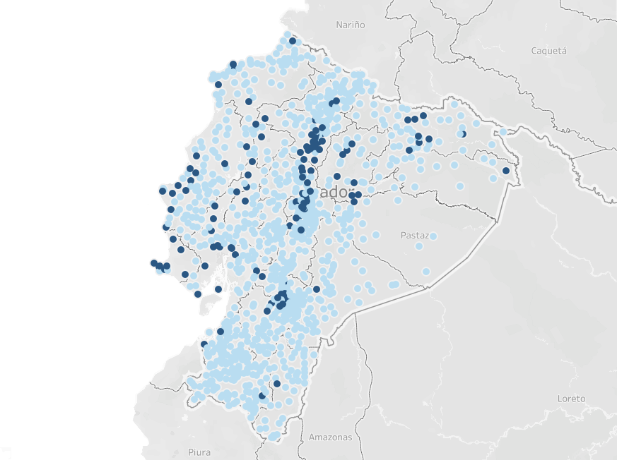
Note: Elaborated in Tableau, showing the detail of the 123 selected parishes relative to the national total.
As observed in the map, the parishes are not exclusively concentrated in a single zone, province, or city. However, they are more frequent around the north-central highlands (sierra) and the southwestern coast, with a relatively smaller number concentrated in the northeastern Amazon. Nevertheless, the distribution is not exclusive to any single region of the country. Furthermore, it is appropriate to compare the poverty distributions between the total population and the study sample; figure 2 shows the poverty distribution of the total population, while figure 3 presents separate distributions for the parishes included and excluded from the study.
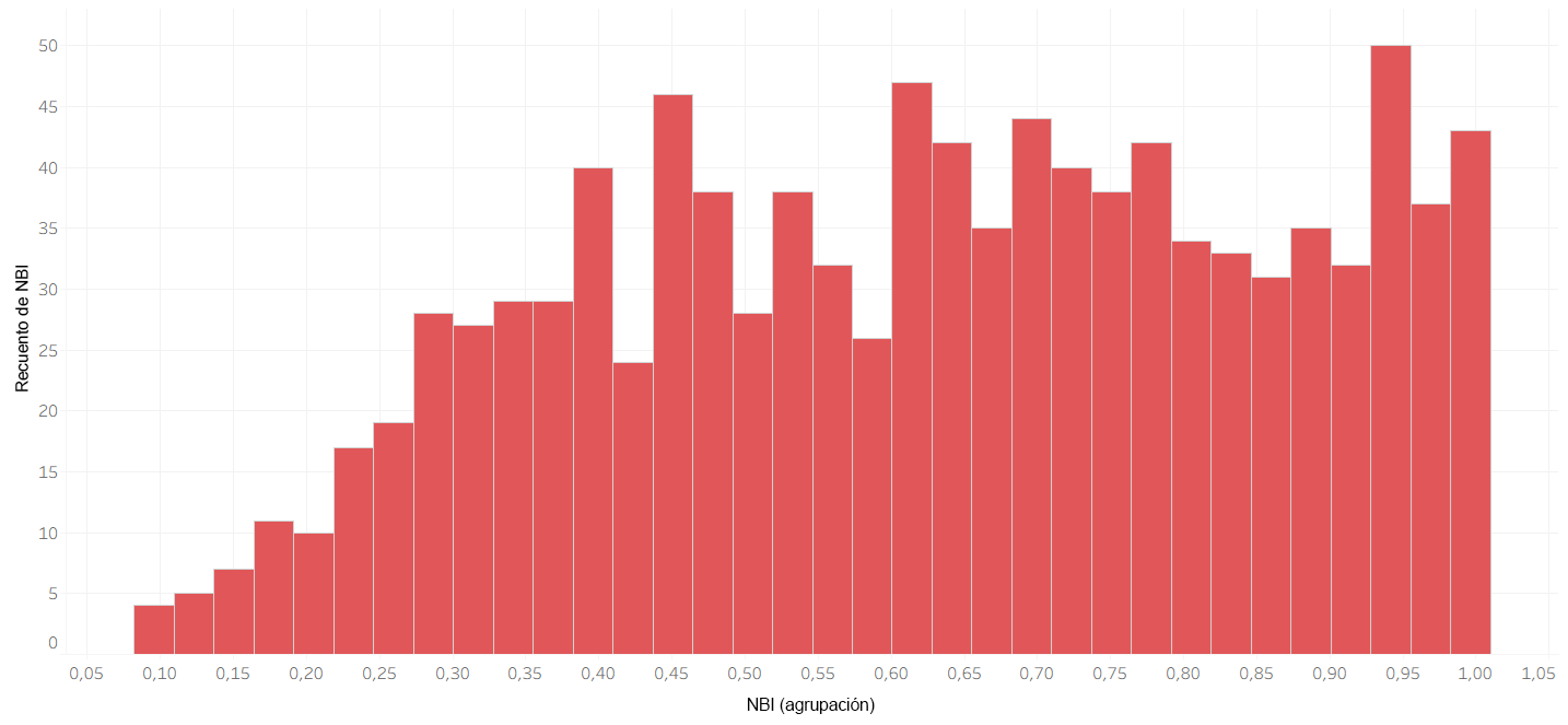
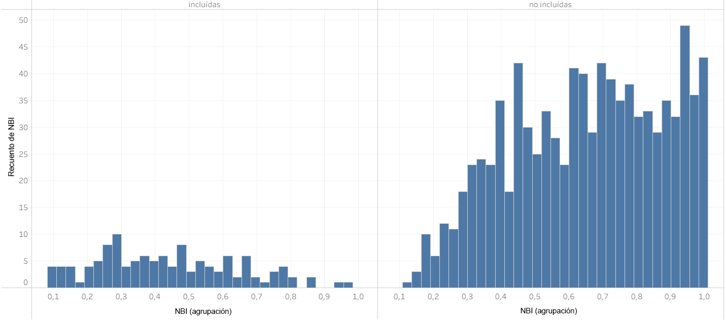
It can be observed that in both the total population and the excluded group, there is a clear left-skewed distribution, revealing a pronounced presence of poverty in the country. In the case of the included parishes, there is a better balance. While this is useful for drawing inferences, it limits the extent to which results from the study sample can be generalized to the entire country. The population variance of the NBI variable is \(\approx 0.05\) (resulting in a standard deviation of \(\approx 0.23\)), whereas the variance for the study sample is \(\approx 0.04\) (standard deviation of \(\approx 0.2\)). This indicates that the selected sample maintains a high diversity of poverty values, even though they are relatively lower than those of the total population.
The fact that our sample has a lower mean poverty level than the overall NBI makes sense, as this is where data availability was highest. It is likely that areas with higher poverty suffer from greater infrastructure deficiencies, which limits data collection and labeling. Finally, it is pertinent to compare the concentration of urban variables in our sample to determine if they are well-balanced or overly concentrated. Nevertheless, despite their limitations, the data allow for the extraction of important conclusions. In this context, it appears preferable to analyze the available data rather than refrain from analysis altogether.
3.2 Models
3.2.1 Variable Transformation
From the initial set of columns available in the dataset, 15 candidate variables were identified with the potential to explain variations in poverty. To better understand their statistical properties, an exploratory analysis of the variable distributions was conducted using histograms (see figure 4). This visual inspection revealed a marked disparity in the scales of the variables, as well as the presence of clustering. Such characteristics can negatively affect the performance and interpretability of models, especially those that assume linear relationships, as is the case in this study.
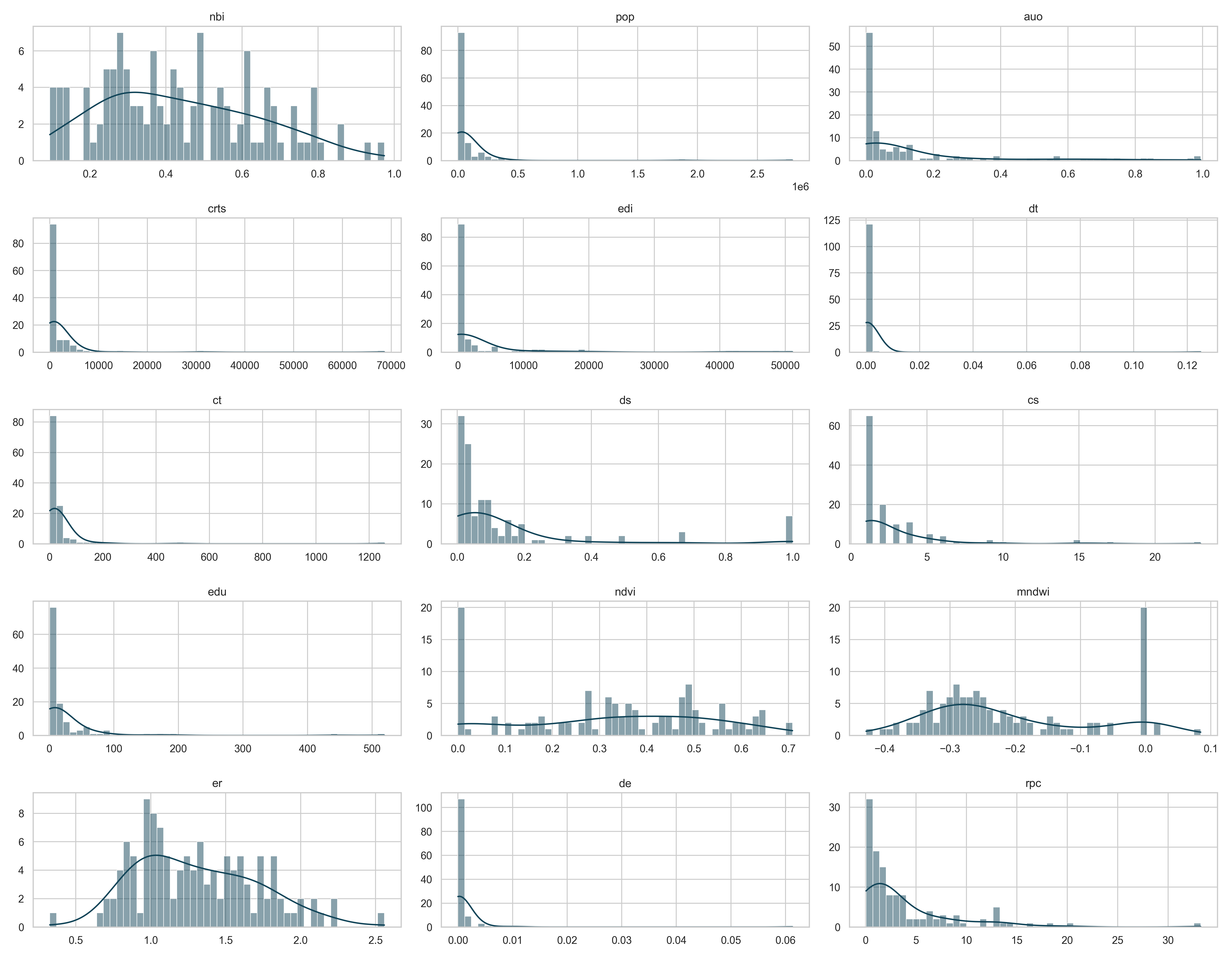
Note: The y-axis shows the frequency of each variable, and the x-axis shows their intervals.
Consequently, natural logarithmic transformations were applied to the variables that required scale adjustment. These transformed variables are denoted by adding the prefix “log_” to the original variable name; for example, \(log\_pop\) refers to \(\ln(pop)\). The adjusted distributions are shown below (see figure 5). Logarithmic transformation is a common technique used to reduce skewness, stabilize variance, and linearize relationships between variables. By compressing the scale of variables with large values and expanding those concentrated near zero, this transformation tends to produce more symmetric variables that are closer to a normal distribution, thereby enhancing the robustness and interpretability of regression models.
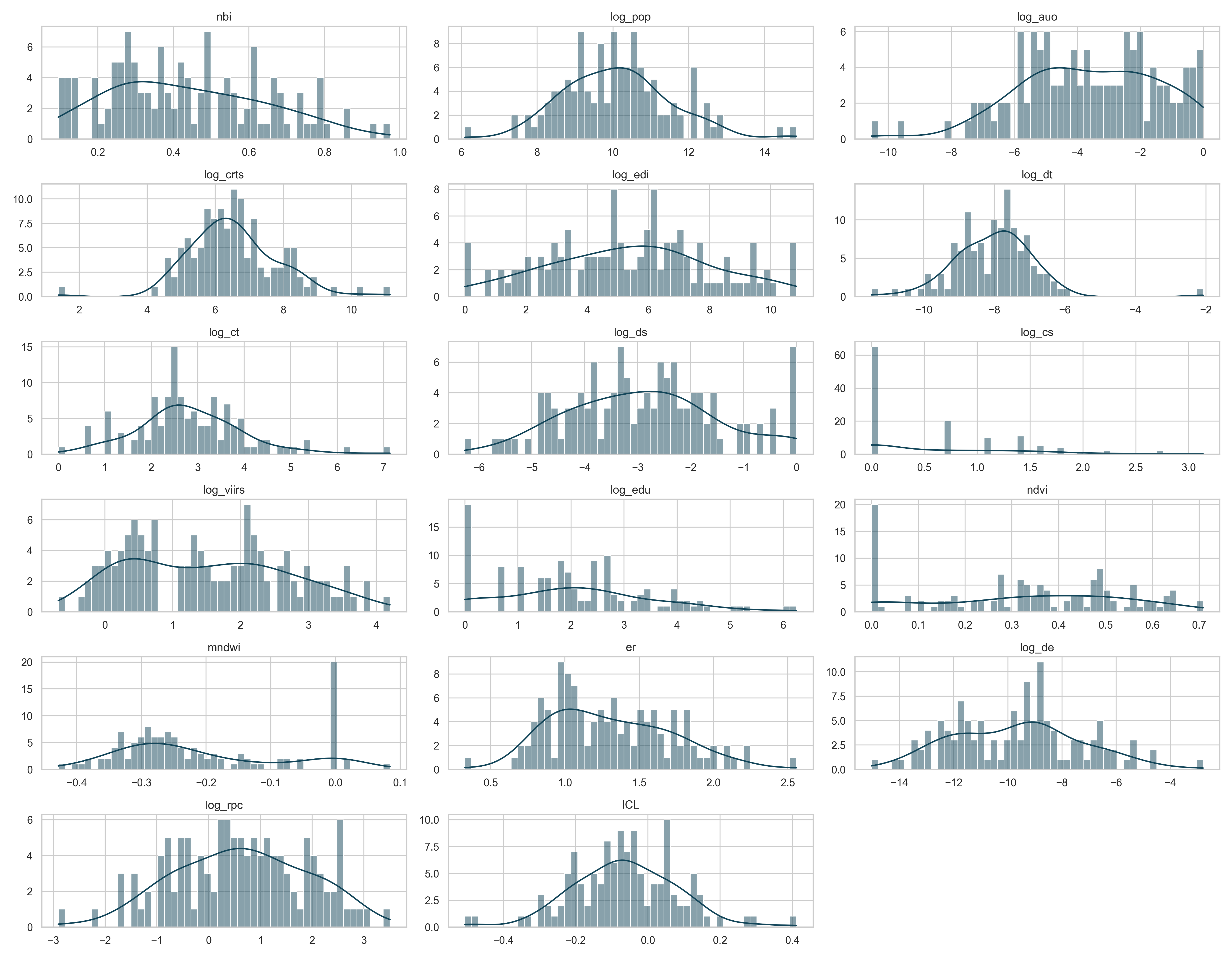
Note: The x-axis displays the intervals of the NBI variable.
3.2.2 Variable Selection and Specification
Seven variable selection methods were employed to specify regressions where the dependent variable is \(nbi\). Each model specification corresponds to the linear combination of variables selected by each method, plus a constant term. table 2 presents the results of the variable selection process carried out using seven distinct methodologies, each grounded in different statistical or machine learning frameworks.
| Method | Variables | Model |
|---|---|---|
| Backward Selection | \(er\), \(log\_auo\), \(log\_crts\), \(log\_ct\), \(ICL\), \(ndvi\), \(mndwi\), \(log\_edu\), \(log\_de\), \(log\_ds\), \(log\_pop\), \(log\_cs\), \(log\_viirs\), \(log\_dt\) | 1 |
| Forward Selection | \(log\_pop\), \(log\_auo\), \(log\_crts\), \(log\_ct\), \(log\_ds\), \(log\_cs\), \(log\_viirs\), \(log\_edu\), \(ndvi\), \(mndwi\), \(er\), \(log\_de\), \(ICL\) | 2 |
| Lasso and ElasticNetCV Regularization | \(log\_auo\), \(log\_crts\), \(log\_dt\), \(log\_ct\), \(log\_ds\), \(log\_viirs\), \(log\_edu\), \(er\) | 3 |
| Recursive Feature Elimination (RFE) | \(log\_ct\), \(log\_viirs\), \(ndvi\), \(mndwi\), \(er\) | 4 |
| Tree-based Feature Importance | \(log\_pop\), \(log\_auo\), \(log\_crts\), \(log\_dt\), \(log\_ct\), \(log\_ds\), \(log\_cs\), \(log\_viirs\), \(log\_edu\), \(ndvi\), \(mndwi\), \(er\), \(log\_de\), \(ICL\) | 5 |
| SelectKBest | \(log\_pop\), \(log\_auo\), \(log\_crts\), \(log\_viirs\), \(log\_edu\), \(ndvi\), \(er\) | 6 |
| Boruta | \(log\_auo\), \(log\_viirs\), \(mndwi\), \(er\) | 7 |
The backward selection method starts from the full set of candidate variables and iteratively removes the predictor with the lowest statistical significance at each step. This procedure retained a relatively large set of predictors, including indicators of infrastructure (\(log\_ct\), \(log\_crts\), \(log\_ds\), \(log\_cs\), \(log\_de\), \(ICL\)), economic activity (\(log\_viirs\)), environmental conditions (\(ndvi\), \(mndwi\)), and demographic and labor variables (\(log\_pop\), \(er\)).
In contrast, the forward selection method begins with an empty model and progressively incorporates the variables that generate the greatest improvement in model fit. Under this approach, a diverse set of covariates was selected, combining proxies for urbanization and economic activity (\(log\_ct\), \(log\_auo\), \(log\_de\), \(log\_viirs\)), environmental indicators (\(ndvi\), \(mndwi\)), and labor variables (\(er\)).
On the other hand, the Lasso and ElasticNetCV regularization methods introduce penalties on the model coefficients in order to reduce complexity and address multicollinearity. This approach selected a smaller subset of variables than the previous two methods, highlighting measures of urban infrastructure (\(log\_ct\), \(log\_crts\), \(log\_ds\), \(log\_dt\)), economic activity (\(log\_viirs\)), and employment (\(er\)).
For both Lasso and ElasticNetCV, a five-fold cross-validation scheme was employed. In the case of ElasticNetCV, a predefined grid of \(l1\_ratio\) values \([0.1, 0.5, 0.7, 0.9, 0.95, 0.99, 1]\) was considered. In both models, the regularization parameter was selected automatically via cross-validation, and variables with non-zero coefficients were retained for subsequent analysis.
The RFE method selects variables by recursively removing those with the lowest relative importance according to model performance. This procedure identified five key predictors: \(log\_ct\), \(log\_viirs\), \(ndvi\), \(mndwi\), and \(er\), capturing dimensions of urbanization, economic activity, environmental conditions, and employment. The underlying algorithm was based on an ordinary least squares linear regression framework targeting a fixed subset of five optimal features. Variables were iteratively eliminated based on the statistical magnitude and significance of their estimated coefficients.
The tree-based feature importance approach uses decision tree ensembles to evaluate the relative contribution of each variable to the model’s overall explanatory power. The results highlight the importance of variables associated with urbanization and infrastructure (\(log\_ct\), \(log\_crts\), \(log\_dt\), \(log\_ds\), \(log\_cs\), \(ICL\)), economic activity (\(log\_viirs\)), educational services (\(log\_edu\)), environmental indicators (\(ndvi\), \(mndwi\)), and labor and institutional conditions (\(log\_de\)). A random forest regression architecture was implemented, where variables were ranked according to their mean decrease in impurity, prioritizing those that maximize the reduction of residual variance across the estimated trees.
The SelectKBest method evaluates each variable independently using univariate statistical tests and selects those with the highest explanatory power, given a fixed number of predictors. Configured to retain the seven most relevant variables, this method selected indicators of economic activity (\(log\_viirs\)), urbanization (\(log\_auo\), \(log\_crts\)), environmental conditions (\(ndvi\)), educational services (\(log\_edu\)), and employment (\(er\)). The selection utilized univariate linear regression tests, prioritizing variables that exhibited the highest \(F\)-scores and lowest \(p\)-values.
Finally, the Boruta algorithm is a robust ensemble-based method that identifies relevant variables by comparing their structural importance against randomized reference attributes. This approach selected a reduced set of predictors—\(log\_auo\), \(log\_viirs\), \(mndwi\), and \(er\)—representing metrics of urbanization level, economic activity, environmental conditions, and employment. The selection mechanism relied on an iterative random forest procedure, statistically testing variable importance against permuted shadow features to ensure that only significantly relevant predictors were retained in the final specification.
3.3 Assumption Testing
For the specified regression models,, it is essential to verify that the classical assumptions underlying linear regression are adequately met to ensure the validity of statistical inferences, unbiasedness of estimators, and the overall reliability of the models. The following standard assumptions were systematically tested:
linearity;
independence of errors;
homoscedasticity;
normality of residuals; and
no multicollinearity among independent variables.
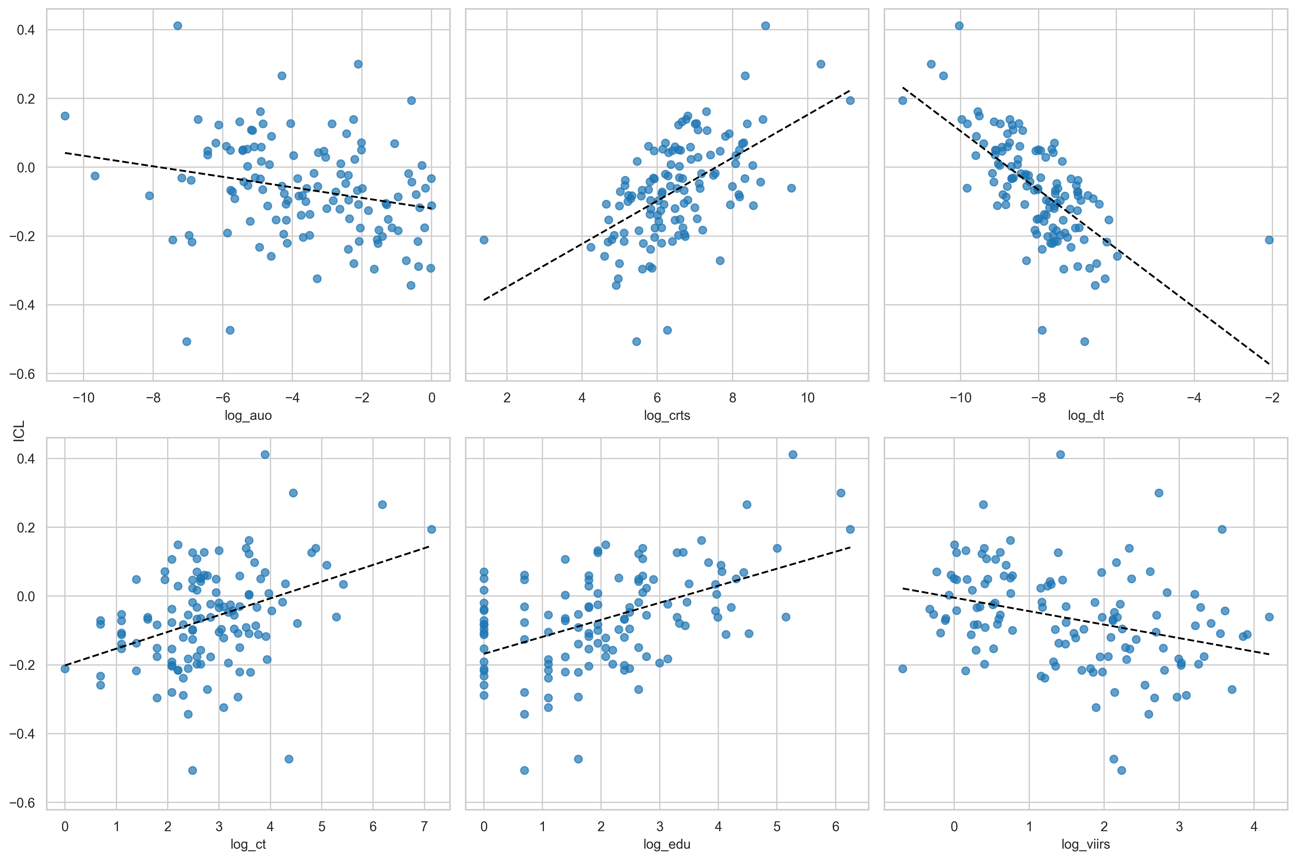
Linearity was assessed graphically, as shown in figure 6. Since logarithmic transformations were applied, the relationships that remain to be verified are those of the variables not log-transformed. These, in fact, exhibit linear relationships.
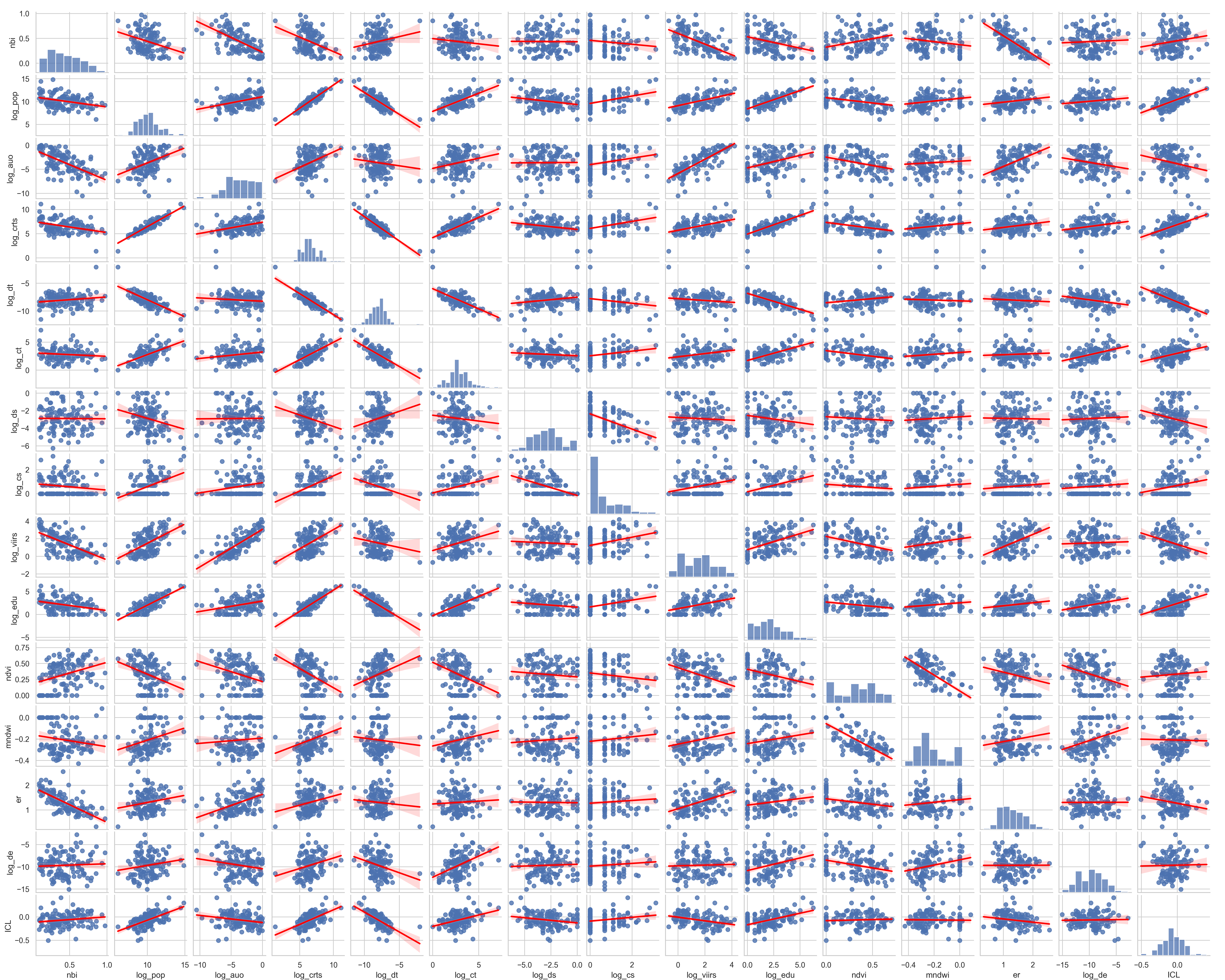
The remaining classical assumptions were evaluated using formal statistical tests selected for their wide acceptance and diagnostic capacity in regression analysis. table 3 specifies the statistical test employed for each assumption and the threshold used to conduct the corresponding hypothesis test.
| Assumption | Statistical Test | Recommended Threshold |
|---|---|---|
| Independence of errors | Durbin-Watson (DW) | Between 1.5 and 2.5* |
| Homoscedasticity | Breusch-Pagan (BP) | p-value \(>\) 0.05 |
| Normality of residuals | Jarque-Bera (JB) | p-value \(>\) 0.05 |
| No multicollinearity | Variance inflation factor (VIF) | VIF \(<\) 10 (ideally \(<\) 5) |
Note: (*) In fact, the goal is for the value to be close to 2 in the ideal scenario, which indicates that the residuals are independent and that there are no correlation patterns among them. However, in practice, this interval is used.
Following the implementation of these diagnostic tests, the results revealed that the models do not fully satisfy all classical assumptions. table 4 provides a concise summary of the specific assumption violations or concerns detected for each model. Additionally, this table reports the results of the overall model significance tests through the F-test, including both the p-value and the F-statistic. These metrics help evaluate whether the explanatory variables jointly contribute significantly to explaining the variance of the dependent variable and thus assess the overall explanatory power and adequacy of each specified model.
| Model | DW | BP | JB p | Max VIF | F-stat | F p-val |
|---|---|---|---|---|---|---|
| 1 | 1.75 ✅ | 0.482 ✅ | 0.728 ✅ | 667.21 ❌ | 16.61 ✅ | 0.000 ✅ |
| 2 | 1.74 ✅ | 0.663 ✅ | 0.714 ✅ | 432.49 ❌ | 18.05 ✅ | 0.000 ✅ |
| 3 | 1.74 ✅ | 0.663 ✅ | 0.714 ✅ | 432.49 ✅ | 18.05 ✅ | 0.000 ✅ |
| 4 | 1.62 ✅ | 0.527 ✅ | 0.856 ✅ | 9.17 ❌ | 41.17 ✅ | 0.0000 ✅ |
| 5 | 1.75 ✅ | 0.482 ✅ | 0.728 ✅ | 667.21 ❌ | 16.61 ✅ | 0.000 ✅ |
| 6 | 1.65 ✅ | 0.217 ✅ | 0.660 ✅ | 319.87 ❌ | 31.28 ✅ | 0.000 ✅ |
| 7 | 1.63 ✅ | 0.280 ✅ | 0.638 ✅ | 10.06 ✅ | 52.77 ✅ | 0.000 ✅ |
Validation criteria: \(1.5 \leq DW \leq 2.5\), \(BP > 0.05\), \(JB > 0.05\), \(\text{Max VIF} < 10\), high F-statistic, and \(\text{F p-val} < 0.01\).
Although all models pass the normality and homoskedasticity tests, there is a critical issue of severe multicollinearity in models 1, 2, 3, 5, and 6 (VIF \(> 300\)). This makes their coefficients unstable and unreliable. Models 4 and 7 substantially mitigate this problem, reducing the VIF to much more manageable levels (\(\approx 9\)–\(10\)) and improving overall model fit (F-statistic).
The model exhibits a satisfactory overall fit, as can be seen in the results reported in table 5, with a coefficient of determination (\(R^2\)) of 0.638, indicating that the independent variables explain 63.8% of the variability in NBI. The overall significance of the model was confirmed by the F-statistic (\(F = 47.37\), \(p < 0.001\)).
Note: Standard errors are by default heteroscedasticity-robust (HC1).
Regarding the individual coefficients, logarithmic nighttime light intensity (\(log\_viirs\)) shows a negative and statistically significant relationship at the 1% level (\(p < 0.001\)), suggesting that areas with higher luminous activity tend to exhibit lower levels of NBI. Similarly, the variable \(er\) presents a negative and highly significant coefficient (\(\beta = -0.288\), \(p < 0.001\)). In contrast, the vegetation index (\(ndvi\)) displays a positive and statistically significant association at the 5% level (\(\beta = 0.225\), \(p = 0.014\)).
It is worth noting that the control variables \(log\_ct\) and \(mndwi\) are not statistically significant (\(p > 0.05\)); therefore, there is insufficient evidence to conclude that they influence the dependent variable in this specification.
3.4 Spatial Autocorrelation and Spatial Error Model
Given the spatial nature of the data, in which the units of observation correspond to geographically defined parishes, spatial autocorrelation may be present. To formally test for its existence, a spatial autocorrelation test based on Moran’s I index was applied. Moran’s I is a widely used statistical measure to identify patterns of spatial dependence. This index generally takes values between \(-1\) and \(1\): values close to zero indicate the absence of spatial autocorrelation, positive values reflect the presence of spatial clustering of similar values, and negative values suggest spatial dispersion patterns.
The estimated value of Moran’s I was \(0.217\), accompanied by a highly significant \(p\)-value (\(p = 0.018\)), implying that the observed pattern is not random and that there is a \(98.2\%\) level of confidence. This result provides evidence of positive spatial autocorrelation of weak-to-moderate magnitude, indicating that geographically proximate parishes tend to exhibit residuals with similar values more frequently than would be expected under a random process. Consequently, the classical assumption of error independence is violated due to the presence of underlying spatial patterns, and ignoring this dependence may compromise both the validity of statistical inference and the precision of the estimators.
In light of this evidence, a spatial error model (SEM) was estimated. This model extends the classical linear regression framework by explicitly incorporating the spatial structure into the error term. This approach allows for capturing and correcting unobserved spatial dependence in the residuals, thereby improving model specification and the robustness of the resulting conclusions.
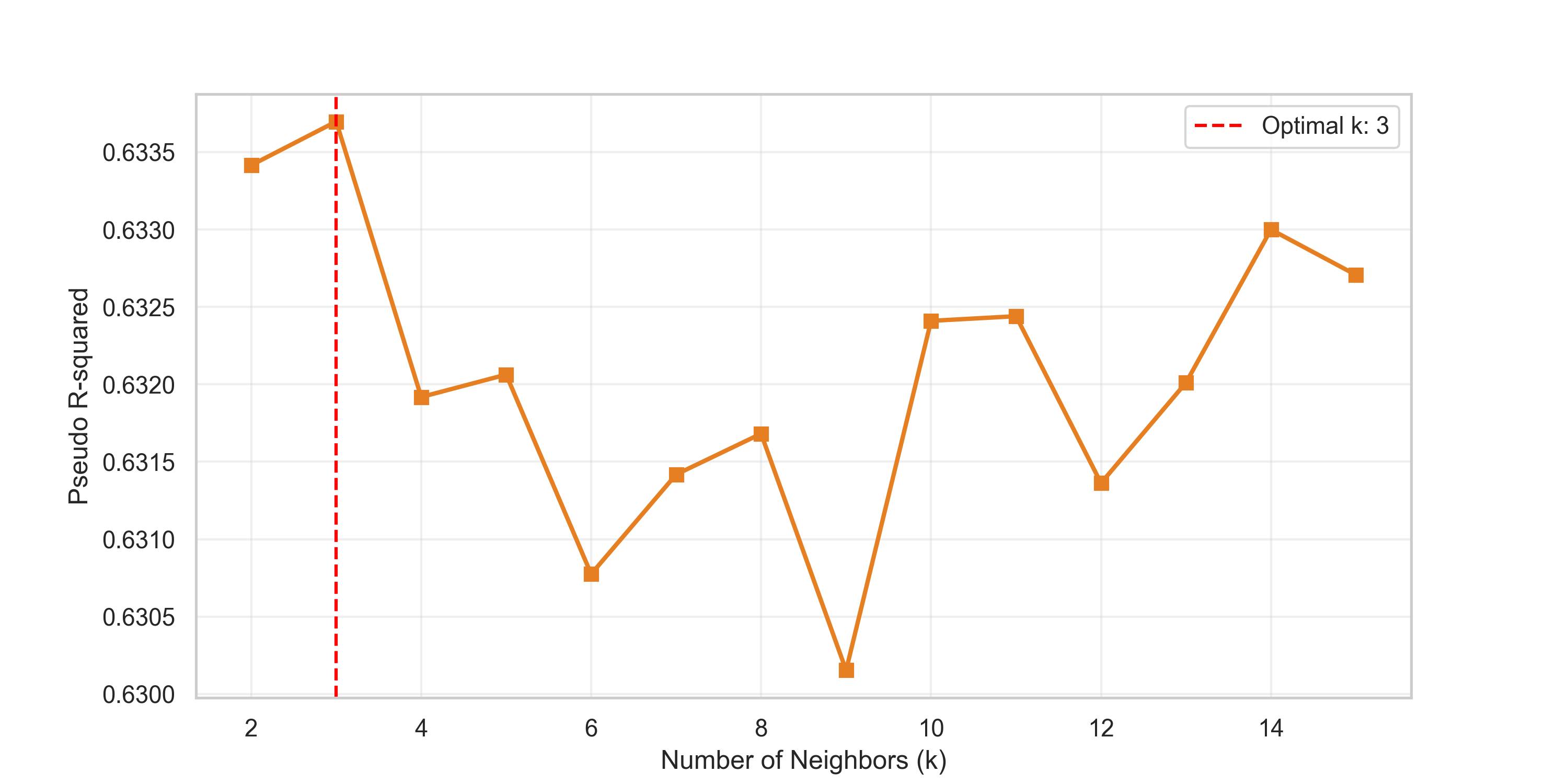
The SEM requires a spatial weights matrix, which reflects the geographical neighborhood structure by assigning weights to nearby observations that may influence one another. By incorporating this matrix into the SEM formulation, the model explicitly accounts for how spatial autocorrelation affects the error term, allowing for a better model fit. The matrix was constructed using a \(k\)-nearest neighbors approach. The optimal number of neighbors was determined by iterating through a range of \(k\) values (\(k \in [2, 15]\)) and selecting the one that maximized the pseudo R-squared of the GM error model. The optimal result corresponded to three nearest neighbors. The outcome of this exercise is illustrated in figure 7.
Therefore, the SEM was specified using a 3-nearest-neighbors spatial weights matrix: \[nbi = \beta_0 + \beta_1 \cdot log\_viirs + \beta_2 \cdot ndvi + \beta_3 \cdot mndwi + \beta_4 \cdot er + \epsilon,\]
where \(\epsilon = \lambda W \epsilon + u\). \(W\) is the spatial weights matrix and \(\lambda\) is the spatial autoregressive parameter in the error term.
The estimation was conducted using the generalized method of moments (GM) with spatially weighted least squares to correct for spatial autocorrelation and the heteroskedasticity inherent in the geographic NBI data. Unlike maximum likelihood methods, the GM approach provides greater robustness by not requiring the assumption of normally distributed errors, allowing for consistent and efficient estimation of the spatial interaction parameter (\(\lambda\)) and the coefficients of the explanatory variables.
4 Results and Limitations
The results of the model, presented in table 6, indicate a satisfactory overall fit, with a pseudo \(R^2\) of 0.6337, suggesting that the model explains 63.3% of the variability in the NBI variable.
| Panel A: Parameter Estimates | ||||
|---|---|---|---|---|
| Variable | Coefficient | Std. Error | \(z\)-Statistic | \(p\)-value |
| Constant | 0.85320 | 0.06467 | 13.19368 | 0.00000 |
| log_ct | 0.00884 | 0.01094 | 0.80839 | 0.41887 |
| log_viirs | -0.06450 | 0.01263 | -5.10654 | 0.00000 |
| ndvi | 0.16276 | 0.11078 | 1.46918 | 0.14178 |
| mndwi | 0.18908 | 0.16114 | 1.17339 | 0.24064 |
| er | -0.27559 | 0.03644 | -7.56242 | 0.00000 |
| \(\lambda\) | 0.31242 | |||
| Panel B: Model Diagnostics | ||||
| Observations | 123 | |||
| Dependent variable | NBI | |||
| Mean dependent var. | 0.4366 | |||
| Std. dependent var. | 0.2079 | |||
| Pseudo \(R^{2}\) | 0.6337 | |||
| Degrees of freedom | 117 |
4.1 Analysis of Statistically Significant Predictors
Elasticity of economic activity (\(\text{log\_viirs}\)): The coefficient associated with radiance (\(\beta = -0.06450\); \(p < 0.001\)), a proxy for economic activity, demonstrates a negative and highly significant impact on NBI. Under this log-linear specification, the result suggests that increases in radiance are associated with a modest reduction in poverty.
Impact of the variable \(er\): The variable \(er\) is identified as the determinant with the largest relative magnitude (\(\beta = -0.27559\); \(z = -7.56\)). The strength of its \(z\)-statistic allows us to infer that for each additional unit in \(er\), poverty is reduced by approximately 0.27 units, holding all other variables constant. This coefficient represents the core of the model’s predictive capacity.
Spatial interaction parameter (\(\lambda\)): The estimation yielded a value of \(\lambda = 0.31242\). The positive magnitude of this parameter confirms the existence of diffusion processes and territorial dependence. Poverty in a parish is not independent of its surroundings; rather, there is a contiguity effect: neighboring parishes tend to share poverty patterns that are not explained by the included variables. This finding justifies the use of a SEM, which corrects for residual autocorrelation and prevents biased estimates. Furthermore, it confirms that poverty is not randomly distributed; there is spatial dependence in the errors. This indicates that unobserved factors that increase poverty in one parish are likely to affect neighboring parishes as well.
4.2 Non-Significant Variables
Environmental factors (\(ndvi\) and \(mndwi\)) did not show a statistically significant association (\(p > 0.05\)), suggesting that at this scale and neighborhood configuration, biophysical conditions do not directly explain variations in poverty. This implies that environmental variability alone does not constitute a determinant of structural poverty once economic development factors and spatial structure are controlled for. Likewise, the variable \(log\_ct\) (\(p = 0.4188\)) does not provide sufficient statistical evidence to reject the null hypothesis of no effect on NBI, indicating that road infrastructure alone is not associated with poverty reduction.
4.3 Discussion
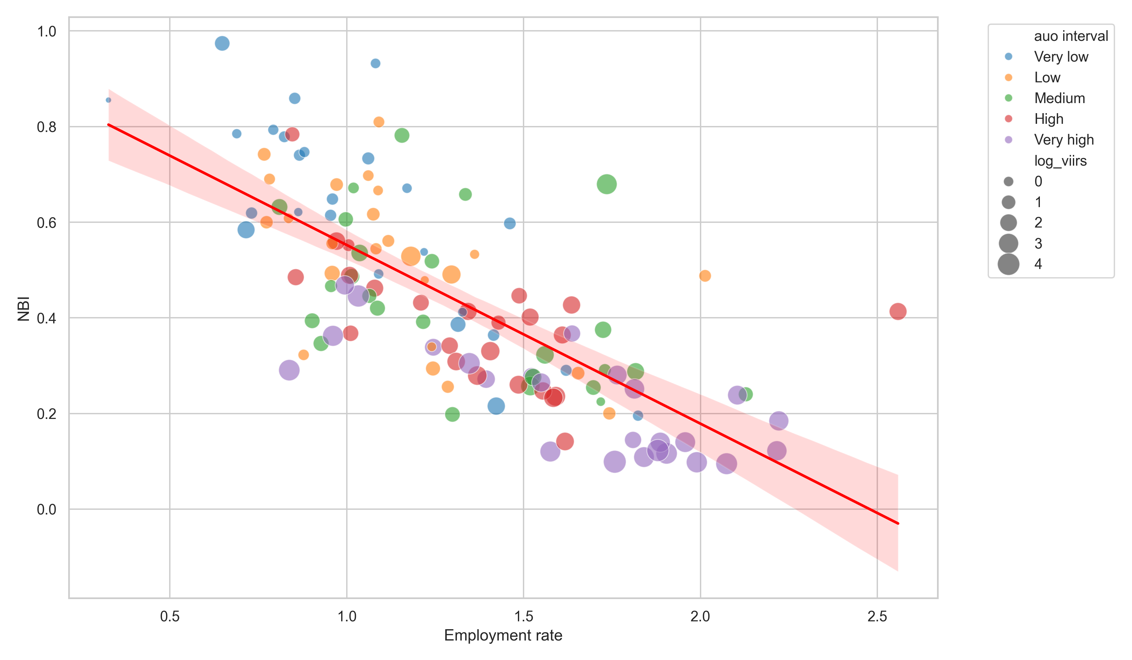
Parishes with higher employment rates tend to be the most urbanized, as can be seen in the figure 8 below. The color of the spheres corresponds to the interval classifying the percentage of urban land (\(auo\)) in the parishes; additionally, the size of the spheres represents the logarithm of radiance. This pattern summarizes the results but raises further questions: for example, to what extent is the level of urbanization related to employment, economic activity, and poverty?
4.3.1 The ICL as a Summary of Urbanization
When comparing the ICL with the logarithms of the variables \(auo\) and \(log\_crts\), their relationships remain consistent. A higher percentage of urban land is inversely related to per capita luminous consumption adjusted for urban areas and buildings (see figure 9).
On the other hand, if we focus on the variables \(log\_ct\) and \(log\_dt\), this consistency is preserved. The observed relationship between the consumption index and the structure of the road network suggests a dynamic of systemic efficiency rather than mere infrastructure availability.
Road network density (\(dt\)) and consumption: The negative correlation observed between the logarithm of road density (\(log\_dt\)) and the consumption index suggests that per capita consumption efficiency is optimized in denser network structures. From graph theory, higher density implies a reduction in the “average path” between nodes, which could suggest lower transaction and transportation costs, allowing for more efficient per capita electricity consumption.
Network components (\(ct\)): The interpretation of components can follow the following criteria:
One component: The entire road network is connected. One can travel from any point to another. Ideal.
Few components: There are some isolated areas (e.g., islands, rural roads). This may be normal.
Many components: The network is highly fragmented. There are many roads or sectors without connection to the rest. This may indicate problems with connectivity or data quality.
In this regard, the variable \(ct\), which represents the constituent elements of the road graph (nodes, edges, and their connectivity), shows a positive relationship with consumption. This may indicate the effect of network complexity: as the road graph acquires more components and higher connectivity (transitioning from dendritic structures to meshes), economies of scale arise that drive consumption. However, in the spatial regression model, this variable did not reach statistical significance (\(p = 0.418\)), indicating that, although there is a visual correlation, the effect is absorbed by other stronger variables such as nighttime luminosity or spatial density.
Moreover, when comparing the index with the logarithms of the number of school institutions (\(edu\)) and radiance, we obtain direct and inverse relationships, respectively. It would be interesting to investigate why a greater presence of schools is associated with a higher ICL.
The previous comparative analysis of relationships invites considering the index as an indirect measure of urbanization.
4.3.2 Study Limitations
This study presents important limitations. First, data coverage was not complete. As noted, data could be used for only 123 out of 1042 parishes (\(11.80\%\)). In addition, some variables—such as the number of educational establishments, buildings, and service networks—were drawn from collaborative OpenStreetMap databases, where quality depends on voluntary user tagging.
Lastly, the static analysis for the year 2022 does not allow for establishing causal relationships or temporal dynamics. Future research could incorporate multi-year panel data or analyze specific shocks such as the COVID-19 pandemic.
4.3.3 Policy Implications
The results suggest considering short-term interventions focused on employment and production, since infrastructure improvement policies alone, without accompanying labor and productivity enhancements, appear to have no lasting effects. Nevertheless, policies aimed at improving infrastructure can promote productivity and growth. An integrated territorial development policy that combines increases and improvements in road connectivity, basic services, and energy efficiency could generate multiplier effects on well-being.
Furthermore, the use of satellite data and open sources allows for the construction of low-cost, wide-coverage territorial monitoring and alert systems. Local and national authorities could leverage this approach to identify critical areas without having to wait for the results of traditional surveys.
5 Conclusions and Discussion
The proposed model explains approximately 63% of the variability in the parish-level poverty rate measured by unmet basic needs. Radiance and employment have reducing effects on poverty, being mild (6%) and substantial (27.5%), respectively.
Additionally, evidence of diffusion processes and territorial dependence of poverty was found. Poverty in a parish is not independent of its surroundings; rather, it tends to share patterns with neighboring parishes that are not explained by the variables included in the model.
Environmental factors did not show a statistically significant association (\(p > 0.05\)), suggesting that, at the parish level and with corrections for spatial dependence, biophysical conditions do not directly explain variations in poverty. This implies that environmental variability alone does not constitute a determinant of structural poverty once economic development factors and spatial structure are controlled for. Similarly, road infrastructure (\(p = 0.4188\) for the logarithm of road network components, which indicates the degree of connectivity among parishes) does not provide sufficient statistical evidence to reject the null hypothesis of no effect on poverty, indicating that road infrastructure alone is not associated with poverty reduction.
Finally, as part of the analysis, a Light Consumption Index (abbreviated as ICL) was constructed, which proves useful for describing the degree of urbanization, as it at least shows coherence with variables accounting for infrastructure and urban expansion.
Acknowledgements
To Alexis Muela, who reviewed the manuscript on multiple occasions, offered relevant insights, and contributed to its translation.
Code availability
The code used for both data extraction and modeling can be reviewed, reproduced, and verified in the GitHub repository Michaeljo112.
References
Aggarwal, S. (2018). Do rural roads create pathways out of poverty? Evidence from india. Journal of Development Economics, 133, 375–395. https://doi.org/https://doi.org/10.1016/j.jdeveco.2018.01.004
Andreano, M. S., Benedetti, R., Piersimoni, F., & Savio, G. (2021). Mapping poverty of latin american and caribbean countries from heaven through night-light satellite images. Social Indicators Research, 156, 533–562. https://doi.org/10.1007/s11205-020-02267-1
Asher, S., & Novosad, P. (2020). Rural roads and local economic development. American Economic Review, 110(3), 797–823. https://doi.org/10.1257/aer.20180268
Donaldson, D. (2018). Railroads of the raj: Estimating the impact of transportation infrastructure. American Economic Review, 108(4-5), 899–934. https://doi.org/10.1257/aer.20101199
Economic Commission for Latin America and the Caribbean. (2007). La medida de necesidades básicas insatisfechas (NBI) como instrumento de medición de la pobreza y focalización de programas (Estudios y Perspectivas - Oficina de La CEPAL En Bogotá LC/L.2840-P). Comisión Económica para América Latina y el Caribe. https://www.cepal.org/es/publicaciones/3544-la-medida-necesidades-basicas-insatisfechas-nbi-instrumento-medicion-la-pobreza
Economic Commission for Latin America and the Caribbean. (2024). América Latina y el Caribe: perfil regional social-demográfico. https://statistics.cepal.org/portal/cepalstat/perfil-regional.html?theme=1&lang=es
Elvidge, C. D., Sutton, P. C., Ghosh, T., Tuttle, B. T., Baugh, K. E., Bhaduri, B., & Bright, E. (2009). A global poverty map derived from satellite data. Computers & Geosciences, 35(8), 1652–1660. https://doi.org/10.1016/j.cageo.2009.01.009
Jean, N., Burke, M., Xie, M., Davis, W. M. A., Lobell, D. B., & Ermon, S. (2016). Combining satellite imagery and machine learning to predict poverty. Science, 353(6301), 790–794. https://doi.org/10.1126/science.aaf7894
Li, M., Lin, J., Ji, Z., Chen, K., & Liu, J. (2023). Evaluación de la pobreza a escala de cuadrícula mediante la integración de luz nocturna de alta resolución y big data espacial: Un estudio de caso en el delta del río pearl. Remote Sensing, 15(18), 4618. https://doi.org/10.3390/rs15184618
Masaki, T., Newhouse, D., Silwal, A. R., Bedada, A., & Engstrom, R. (2020). Small area estimation of non-monetary poverty with geospatial data (Policy Research Working Paper No. 9383). World Bank. https://openknowledge.worldbank.org/server/api/core/bitstreams/9d4473f3-104f-5fa4-8758-0e5035dad36e/content
National Institute of Statistics and Censuses. (2023). Ficha metodológica de indicador: Porcentaje de personas u hogares en pobreza por necesidades básicas insatisfechas (NBI) [Ficha Metodológica]. National Institute of Statistics; Censuses. https://www.ecuadorencifras.gob.ec/
National Institute of Statistics and Censuses. (2024). Pobreza por necesidades básicas insatisfechas (NBI): resultados Censo Ecuador [Informe de Resultados]. INEC. https://www.censoecuador.gob.ec/wp-content/uploads/2024/12/Pobreza_NBI_Resultados_Dic2024.pdf
National Institute of Statistics and Censuses. (2025). Encuesta Nacional de Empleo, Desempleo y Subempleo (ENEMDU): Indicadores de pobreza y desigualdad, diciembre 2025 [Boletín Técnico]. INEC. https://www.ecuadorencifras.gob.ec/documentos/web-inec/POBREZA/2025/Diciembre/202512_PobrezayDesigualdad.pdf
Puttanapong, N., Martinez, A., Jr., Bulan, J. A. N., Addawe, M., Durante, R. L., & Martillan, M. (2022). Predicting poverty using geospatial data in thailand. ISPRS International Journal of Geo-Information, 11(5), 293. https://doi.org/10.3390/ijgi11050293
United Nations Office for the Coordination of Humanitarian Affairs. (2024). Ecuador - subnational administrative boundaries. The Humanitarian Data Exchange (HDX). https://data.humdata.org/dataset/cod-ab-ecu
Wang, K., Zhang, L., Cai, M., Liu, L., Wu, H., & Peng, Z. (2023). Measuring urban poverty spatial by remote sensing and social sensing data: A fine-scale empirical study from zhengzhou. Remote Sensing, 15(2), 381. https://doi.org/10.3390/rs15020381
Zhao, X., Yu, B., Liu, Y., Chen, Z., Li, Q., Wang, C., & Wu, J. (2019). Estimation of poverty using random forest regression with multi-source data: A case study in bangladesh. Remote Sensing, 11(4), 375. https://doi.org/10.3390/rs11040375
VIIRS is converted from square centimeters to square meters for comparability with square meters of occupied urban area↩︎