
| Variable | Year | Mean | SD | Min | Max |
|---|---|---|---|---|---|
| Poverty rate (UBN) | 2001 | 87.069% | 0.098 | 46.939% | 100% |
| Poverty rate (UBN) | 2010 | 79.243% | 0.124 | 34.606% | 98.271% |
| Poverty rate (UBN) | 2022 | 61.082% | 0.168 | 12.205% | 96.215% |
| Human capital | 2001 | 5.623 | 1.324 | 2.667 | 9.902 |
| Human capital | 2010 | 7.189 | 1.458 | 3.636 | 11.648 |
| Human capital | 2022 | 9.734 | 1.406 | 5.796 | 13.949 |
| Household size | 2001 | 4.383 | 0.411 | 3.107 | 5.956 |
| Household size | 2010 | 3.903 | 0.403 | 2.944 | 6.007 |
| Household size | 2022 | 3.278 | 0.262 | 2.718 | 4.787 |
| Older adult population | 2001 | 7.263% | 0.025 | 2.627% | 19.526% |
| Older adult population | 2010 | 7.491% | 0.031 | 2.133% | 19.592% |
| Older adult population | 2022 | 9.742% | 0.036 | 2.503% | 21.181% |
| Youth population | 2001 | 20.182% | 0.017 | 13.817% | 23.252% |
| Youth population | 2010 | 19.963% | 0.014 | 15.298% | 23.331% |
| Youth population | 2022 | 19.812% | 0.014 | 15.346% | 23.638% |
| Female-headed households | 2001 | 23.825% | 0.068 | 10.393% | 49.349% |
| Female-headed households | 2010 | 26.815% | 0.060 | 14.902% | 48.270% |
| Female-headed households | 2022 | 36.573% | 0.054 | 20.960% | 51.919% |
| Indigenous population | 2001 | 11.768% | 0.204 | 0% | 93.192% |
| Indigenous population | 2010 | 12.388% | 0.218 | 0% | 97.099% |
| Indigenous population | 2022 | 14.233% | 0.242 | 0% | 97.726% |
| Afro-Ecuadorian population | 2001 | 1.924% | 0.059 | 0% | 54.231% |
| Afro-Ecuadorian population | 2010 | 4.094% | 0.076 | 0.017% | 63.676% |
| Afro-Ecuadorian population | 2022 | 3.483% | 0.105 | 0.043% | 83.966% |
| Population density | 2001 | 87.781 | 230.600 | 0.285 | 3073.340 |
| Population density | 2010 | 105.547 | 285.069 | 0.391 | 3786.630 |
| Population density | 2022 | 124.498 | 339.325 | 0.550 | 4434.890 |
| Primary sector | 2001 | 53.067% | 0.206 | 5.228% | 84.506% |
| Primary sector | 2010 | 48.243% | 0.188 | 2.802% | 82.304% |
| Primary sector | 2022 | 37.513% | 0.175 | 2.926% | 77.010% |
| Secondary sector | 2001 | 12.223% | 0.075 | 2.239% | 57.126% |
| Secondary sector | 2010 | 13.177% | 0.076 | 3.085% | 58.617% |
| Secondary sector | 2022 | 13.876% | 0.070 | 3.538% | 56.533% |
| Tertiary sector | 2001 | 29.797% | 0.139 | 8.550% | 72.018% |
| Tertiary sector | 2010 | 36.432% | 0.145 | 10.074% | 75.634% |
| Tertiary sector | 2022 | 51.749% | 0.135 | 19.798% | 81.227% |
| Informal employment rate | 2001 | 62.248% | 0.067 | 40.744% | 78.810% |
| Informal employment rate | 2010 | 48.276% | 0.078 | 28.504% | 74.301% |
| Informal employment rate | 2022 | 33.573% | 0.086 | 7.548% | 57.004% |
| Emigration | 2001 | 8.314% | 0.075 | 0.119% | 32.742% |
| Emigration | 2010 | 4.556% | 0.039 | 0.435% | 20.362% |
| Emigration | 2022 | 2.148% | 0.029 | 0.097% | 13.868% |
| Retirement income | 2001 | 3.151% | 0.027 | 0.229% | 19.314% |
| Retirement income | 2010 | 3.743% | 0.036 | 0% | 21.533% |
| Retirement income | 2022 | 3.309% | 0.019 | 0% | 9.642% |
| Unemployment rate | 2001 | 1.793% | 0.009 | 0.284% | 6.058% |
| Unemployment rate | 2010 | 9.537% | 0.032 | 3.987% | 19.800% |
| Unemployment rate | 2022 | 20.366% | 0.068 | 8.521% | 59.215% |
7 The Spatial Dimension of Poverty Based on Unsatisfied Basic Needs in Ecuador: A Spatial Panel Approach from 2001 to 2022
Abstract
This paper examines the spatial and temporal dynamics of poverty in Ecuador at the cantonal level over the period 2001-2022. It combines the traditional unsatisfied basic needs (UBN) approach with the CAPECO index to address limitations in the measurement of household economic capacity. The analysis proceeds in four stages: multidimensional poverty measurement, distributional dynamics, exploratory spatial data analysis, and spatial panel econometric modeling. The results reveal a substantial but uneven decline in poverty, with improvements concentrated in housing conditions and school attendance, while access to basic services and economic capacity remain persistent constraints. Spatial analysis uncovers increasing clustering of poverty, with high-high clusters consolidating along the central and northern Coast and low-low clusters in the central-northern Sierra. Distributional dynamics further indicate limited mobility and the presence of territorial poverty traps. Econometric evidence from a Spatial Durbin Model highlights human capital as the most robust driver of poverty reduction, both locally and through spillover effects, whereas unemployment and primary-sector dependence significantly contribute to the persistence and spatial propagation of such poverty. Overall, the findings suggest that poverty in Ecuador is a territorially interdependent phenomenon that requires coordinated regional policies that transcend administrative boundaries.
Keywords
poverty, unsatisfied basic needs, CAPECO index, spatial analysis, regional disparities
1 Introduction
Over the past two decades, poverty, measured through unsatisfied basic needs (UBN), has declined markedly in Ecuador, falling from 65% in 2001 to below 31% in 2023, according to the National Institute of Statistics and Censuses (INEC) (2024a). Despite this aggregate improvement, a growing body of evidence points to pronounced spatial heterogeneity, with poverty exhibiting clear patterns of geographical concentration. Previous research at the cantonal level has documented the presence of spatial clustering and positive spatial autocorrelation, particularly up to 2010 (Orellana Bravo et al., 2018). However, studies conducted at aggregated levels, such as that of provinces, often fail to detect such spatial dependence (García Vélez & Núñez Velázquez, 2022), which suggests that the cantonal scale is more appropriate for capturing territorial dynamics.
From the perspective of economic geography, poverty is not randomly distributed but shaped by structural and spatial processes, including agglomeration forces, labor market segmentation, and unequal access to productive assets. In Ecuador, these mechanisms manifest in persistent territorial disparities, where certain cantons remain trapped in low-development equilibria despite their proximity to dynamic economic centers (Pontarollo et al., 2019). Similar patterns have been documented across Latin America, where poverty tends to cluster geographically and to be influenced by neighboring conditions (Acuña Carrasco et al., 2017; Santos et al., 2017).
In this context, accuracy in the measurement of poverty becomes crucial. While the UBN approach provides a structural perspective on deprivation, it may underestimate economic vulnerability by inadequately capturing household income capacity. To address this limitation, this study incorporates the CAPECO index, which refines the measurement of economic capacity by accounting for educational attainment weighted by labor participation. This adjustment yields a more sensitive identification of economically constrained households.
By building on this measurement framework, the paper analyses the evolution and spatial structure of poverty in Ecuador between 2001 and 2022 using census data for all 221 cantons. The empirical strategy combines distributional analysis, spatial exploratory techniques, and spatial panel econometrics to uncover both temporal dynamics and spatial interdependencies. In doing so, the study seeks to provide a comprehensive account of how poverty evolves across space and time, and to identify the mechanisms that sustain its persistence.
This paper contributes to the literature in three main ways. First, it advances poverty measurement by integrating the CAPECO index into the traditional UBN framework, thereby enabling a more accurate representation of household economic capacity and reducing the risk of underestimating deprivation associated with income constraints. Second, it provides new empirical evidence on the spatial dynamics of poverty at a highly disaggregated level, by combining distributional approaches with spatial econometric techniques. By jointly analyzing mobility, clustering, and spillover effects, the study offers a more comprehensive understanding of territorial inequality. Third, it identifies the key socioeconomic mechanisms underlying the spatial persistence of poverty in Ecuador. In particular, it highlights the central role of human capital in driving poverty reduction and the importance of labor market conditions and productive structure in shaping both local and regional outcomes. These findings have direct implications for the design of place-based policies aimed at reducing structural and spatial inequalities.
Based on this framework, the analysis is guided by four hypotheses. First, incorporating a refined measure of economic capacity reveals higher levels of vulnerability than those captured by the traditional UBN approach. Second, spatial autocorrelation in poverty has strengthened over time and has reinforced the role of geography as a determinant of deprivation. Third, poverty dynamics exhibit limited mobility and have led to the formation of convergence clubs and persistent territorial disparities. Lastly, poverty is shaped not only by local socioeconomic factors but also by spatial spillovers arising from neighboring cantons.
2 Literature Review
The persistence and spatial distribution of poverty have been widely analyzed within the framework of economic geography, which emphasizes the role of spatial interdependence, path dependence, and structural heterogeneity in shaping territorial development outcomes. Rather than being randomly distributed, poverty reflects the interaction between household-level constraints and place-based characteristics, including access to markets, infrastructure, and productive opportunities. The central mechanism highlighted in the literature is that of path dependence, whereby initial conditions exert a long-lasting influence on regional trajectories. In this context, agglomeration theory suggests that economic activity tends to concentrate in already developed areas, thereby generating cumulative advantages that reinforce regional disparities (Bradshaw, 2007). Conversely, peripheral territories may experience shadow effects, whereby proximity to dynamic centers does not translate into spillovers but instead limits local development by attracting resources away from less competitive areas (Aponte et al., 2015). These dynamics are particularly prevalent in developing economies, where uneven spatial development often results in persistent poverty clusters.
Spatial poverty traps emerge when these processes interact with local constraints, such as limited human capital, weak infrastructure, and restricted access to productive assets. Empirical evidence from Latin America indicates that poverty tends to cluster geographically and is significantly influenced by neighboring conditions (Acuña Carrasco et al., 2017; Santos et al., 2017). This implies that poverty is not only a local phenomenon but also a spatially interdependent one, where conditions in adjacent territories shape development outcomes. Consequently, analytical approaches that ignore spatial dependence may lead to biased or incomplete conclusions.
Human capital constitutes a key channel through which these dynamics operate. According to human capital theory (Becker, 1994), education enhances individual productivity and income potential, thereby reducing vulnerability to poverty. However, its effects extend beyond the individual level. At the territorial scale, higher levels of education can generate positive externalities: fostering innovation, improving labor market functioning, and facilitating structural transformation. Conversely, disparities in educational attainment across regions may reinforce spatial inequality by limiting the capacity of lagging areas to attract investment and diversify their productive structure (Jung & Thorbecke, 2003).
Migration and demographic dynamics further reinforce these patterns. Selective migration processes tend to concentrate the more educated and economically active individuals in dynamic regions and hence exacerbate the depletion of human capital in marginalized areas (Wilson, 2012). This mechanism contributes to the persistence of regional disparities, since lagging territories face both structural constraints and a continuous outflow of their most productive population segments. In turn, these processes may interact with demographic structures, such as dependency ratios, thereby amplifying vulnerability in households with limited labor income.
Labor market conditions also play a critical role in shaping poverty outcomes. In contexts characterized by structural heterogeneity, unemployment and informality are not merely cyclical phenomena but reflect persistent mismatches between labor supply and demand (Levernier et al., 2000). Informal employment, while providing short-term income opportunities, often lacks stability and social protection, which limits its capacity to generate sustained improvements in well-being. Moreover, labor market segmentation restricts access to high-productivity sectors, particularly for vulnerable groups, thereby reinforcing income disparities and territorial inequality.
The productive structure of regions further conditions poverty dynamics. A high dependence on primary activities is typically associated with low value added and limited income generation, whereas diversification towards manufacturing and services sectors tends to support inclusive growth (Ravallion & Datt, 1996). In particular, the expansion of the tertiary sector has been identified as a key driver of poverty reduction, since it generates employment opportunities in areas such as education, health, and commerce. However, the benefits of structural transformation are unevenly distributed across space, since they depend on the capacity of regions to integrate into broader economic networks.
Lastly, structural inequalities linked to ethnicity and historical exclusion remain central to understanding poverty in Latin America. Indigenous and Afro-descendant populations often face systemic barriers to accessing education, infrastructure, and formal labor markets, which lead to a territorial concentration of deprivation (Gigler, 2015). These patterns reflect long-standing institutional and social constraints that persist despite overall economic progress. As a result, poverty in these contexts is both socially and spatially embedded, and requires analytical frameworks that account for multiple layers of inequality.
Taken together, this body of literature highlights three key implications for empirical analysis. First, poverty must be understood as a multidimensional and spatially interdependent phenomenon, shaped by both local conditions and interactions with neighboring territories. Second, human capital, labor market dynamics, and productive structure constitute the main channels through which poverty is generated and reproduced across space. Third, spatial econometric approaches are necessary to adequately capture these interdependencies and to prevent biased inference from arising from omitted spatial effects.
By building on these insights, this study adopts a spatial panel econometric framework to examine the determinants and dynamics of poverty at the cantonal level in Ecuador. By explicitly modeling spatial dependence, the analysis captures both direct effects and spillover mechanisms, and provides a more comprehensive understanding of the territorial processes underlying poverty persistence.
2.1 Poverty Measurement
Measuring poverty at the cantonal level requires clear and consistent indicators that reflect the multidimensional nature of deprivation experienced by households. In this study, the cantonal poverty rate is defined as the percentage of households within a canton that suffer deprivation in at least one of the five dimensions captured by the UBN indicator. To ensure robustness, two measurement approaches are adopted. The first approach follows the classic methodology established by the Economic Commission for Latin America and the Caribbean (ECLAC) (2015), which incorporates specific adjustments to the deprivation thresholds to enhance the indicator’s sensitivity and better capture subtle forms of poverty (table 1). The data underpinning this measurement is drawn from Ecuador’s national population censuses for the years 2001, 2010, and 2022, while applying a consistent political-administrative framework of 221 cantons across the entire period (INEC, 2024a).
Two key modifications were made to the classic methodology. First, the UBN measurement conducted by INEC (2024b) in Ecuador considers any household member who has recently engaged in remunerated activity as an income earner, regardless of age.
In other words, this approach would classify a household as non-poor even if none of the adults were employed, as long as several children or adolescents work. In Latin America, child labor is often considered a consequence of poverty (López-Calva, 2006), and evidence supports the link between low income and child labor in the region (Acevedo González et al., 2010; López Ávila, 2009; Noceti, 2011; Río & Cumsille, 2008). To address this issue, our measurement excludes children under 15 years of age from being classified as household income earners in an effort to prevent underestimating poverty caused by failing to take into account its inherent relationship with child labor.
Similarly, regarding the education access dimension, the traditional threshold considers a household poor if it has children aged 12 or younger who do not attend school: this excludes older children from the threshold. In contrast, our measurement slightly extends this threshold to include children up to 15 years of age, thereby increasing the indicator’s sensitivity.
| Dimension | Indicator | Deprivation Threshold |
|---|---|---|
| Household economic capacity | Economic dependency | The head of the household has three or fewer years of schooling and the number of economic dependents exceeds three times the number of income earners who are over 15 years of age. |
| Access to education | School attendance of school-age children | There are children aged 6 to 15 in the household who do not attend school. |
| Housing quality | Housing materials | The floor of the dwelling is made of dirt, sand, or other non-durable materials, and/or the walls are constructed from cane, thatch, or other inadequate materials. |
| Access to basic services | Availability of water and sanitation | A household lacks adequate basic services if it has no proper sanitation system (e.g., sewers, piped water). |
| Overcrowding | Ratio of household members to bedrooms | A household is overcrowded if there are more than three people per bedroom or no dedicated sleeping space. |
Source: Authors’ elaboration based on INEC (Instituto Nacional de Estadística y Censos, 2024b) data.
The second approach to measuring poverty differs from ECLAC’s methodology only in its assessment of the first dimension: household economic capacity. For this dimension, the CAPECO index developed by Gómez et al. (1999) is used, which provides a more appropriate alternative for measurement. The index classifies households into four strata of economic capacity based on the average educational level of all household members, weighted by each member’s status as an income earner. Evidence indicates that, compared to other indicators, CAPECO exhibits the strongest correlation with household per capita income (Álvarez, 2002). Moreover, various applications in Latin America have shown that the index is more sensitive in capturing low economic capacity, and systematically yields higher poverty rates than the classic method (Álvarez, 2002; Mario et al., 2004; Santillán, 2015).
\[CAPECO = \sum_{i = 1}^{n}\frac{{CP}_{i}*{AE}_{i}}{n} \tag{1}\]
where \({CP}_{i}\) takes the value of 1 for employed individuals, 0.75 for retired or pensioned individuals who are not working, and 0 for individuals who are neither employed nor retired; \({AE}_{i}\) denotes the years of education completed in the formal education system; and \(n\) represents the number of household members.
CAPECO classifies household economic capacity according to the following ranges:
| Very low | Low | Medium | High | |
|---|---|---|---|---|
| Ranges | 0 to 1.74 | 1.75 to 2.49 | 2.50 to 4.49 | 4.50 and above |
Source: Gómez et al. (1999).
As shown in table 2, a household is classified as poor according to the UBN in the household economic capacity dimension if its index value falls within the “very low” category (0 to 1.74). Table 3 presents the average cantonal poverty rates and compares the traditional UBN approach with the CAPECO indicator as an alternative for measuring economic capacity. The rates obtained with CAPECO tend to be higher since they more accurately reflect the limitations of household economic capacity. However, the threshold remains conservative because it does not classify households in the “low” economic capacity stratum as poor.
| 2001 | 2010 | 2022 | ||||
|---|---|---|---|---|---|---|
| UBN Traditional | CAPECO | UBN Traditional | CAPECO | UBN Traditional | CAPECO | |
| Mean | 84.52% | 87.07% | 74.19% | 79.24% | 53.11% | 61.08% |
| Median | 87.35% | 89.60% | 87.35% | 80.12% | 51.26% | 60.16% |
| Variance | 0.0127 | 0.0097 | 0.0206 | 0.0154 | 0.0340 | 0.0282 |
Source: Authors’ own elaboration.
Table 4 presents the transition matrix of cantonal poverty rates, grouped into quintiles, for the periods 2001-2010 and 2010-2022. The results show a pronounced persistence in poverty rates, particularly at both ends of the distribution. Cantons with the lowest poverty rates (Q1) exhibit strong immobility: 84.4% remained in the same quintile between 2001 and 2010, and 75.6% did so between 2010 and 2022. Similarly, cantons with the highest poverty rates (Q5) also show remarkable persistence, with 86.4% remaining in Q5 during the first period and 79.6% in the second.
This indicates that cantons with very high or very low poverty rates tend to maintain their relative position over time, which reflects entrenched structural conditions at both ends of the spectrum. By contrast, mobility is more frequent among the intermediate quintiles (Q2-Q4), where a higher share of cantons transition upward or downward, which suggests that relative changes in poverty rates occur predominantly in the middle of the distribution.
Although mobility increased slightly in 2010-2022, especially regarding upward mobility out of Q5 (20.4% transitioned to Q4) and Q1’s movement toward higher quintiles (24.4% combined), the overall pattern still points to a high degree of persistence.
| 2001/2010 | Q1 | Q2 | Q3 | Q4 | Q5 | 2010/2022 | Q1 | Q2 | Q3 | Q4 | Q5 |
|---|---|---|---|---|---|---|---|---|---|---|---|
| Q1 | 84.4 | 15.6 | 0 | 0 | 0 | Q1 | 75.6 | 22.2 | 2.2 | 0 | 0 |
| Q2 | 15.9 | 52.3 | 31.8 | 0 | 0 | Q2 | 20.4 | 47.7 | 29.6 | 2.3 | 0 |
| Q3 | 0 | 22.7 | 47.7 | 29.6 | 0 | Q3 | 4.5 | 27.3 | 56.8 | 11.4 | 0 |
| Q4 | 0 | 9.1 | 20.5 | 56.8 | 13.6 | Q4 | 0 | 2.3 | 11.4 | 65.9 | 20.4 |
| Q5 | 0 | 0 | 0 | 13.6 | 86.4 | Q5 | 0 | 0 | 0 | 20.4 | 79.6 |
Source: Authors’ own elaboration.
According to table 5, between 2001 and 2022, all dimensions of poverty recorded a decline in their average deprivation levels, although the pace and magnitude of improvement varied across dimensions. Regarding the school attendance dimension for children of school age, households experiencing deprivation consistently represented a significantly smaller proportion compared to that of other poverty dimensions during the three years analyzed. The national cantonal average rate stood at 15.69% in 2001, 2.34% in 2010, and 3.53% in 2022, with standard deviations of 4.56%, 1.34%, and 1.9%, respectively. Despite the reduction in standard deviation, the relative dispersion actually increases when the coefficient of variation is considered, which indicates growing inequality among cantons in this deprivation between 2010 and 2022 compared to that of 2001. Furthermore, the increase in the average rate between 2010 and 2022 raises concern, since it suggests a potential underreporting of school dropout among children and youth that the censuses may have failed to fully capture. In contrast, overcrowding showed significant improvement, declining from 33.15% to 20.97% and finally to 10.26%, caused by better housing conditions. Deprivation in physical housing characteristics also progressed steadily, decreasing from 21.92% in 2001 to 17.29% in 2010, and to 10.80% in 2022.
Throughout the period, the highest deprivation levels occurred in access to basic services and economic capacity. Deprivation in basic services fell from 76.02% in 2001 to 67.19% in 2010, and to 46.59% in 2022. This reflects considerable progress while highlighting persistent structural deficits in water and sanitation. The standard deviation (SD) in access to basic services increased from 0.153 in 2001 to 0.165 in 2010, and to 0.198 in 2022, which indicates that, despite average improvements, territorial inequality in this dimension actually rose over time. Regarding economic capacity, deprivation decreased from 45.09% to 39.08%, and then to 27.71%, due to improvements in household income and resources, although a significant portion of the population remained affected. The SD for this dimension remained at approximately 9% throughout the period; combined with the decline in the average, this indicates a relative increase in the dispersion of poverty, meaning inequality among cantons grew regarding this deprivation. As noted, this measurement classified as poor only those households with “very low economic capacity.” To analyze the sensitivity of results to threshold changes, a second measurement was conducted that included households with “low economic capacity,” although this measurement was then excluded from the overall UBN poverty rate calculation. Under the adjusted threshold, the results appear less encouraging: by 2022, an average of 37.16% of households at the cantonal level fell into the low or very low economic capacity category, with increasing dispersion over time (table 5).
Overall, improvements across dimensions were uneven: several cantons in the Sierra achieved faster reductions in overcrowding, improved physical housing characteristics, and access to basic services, while many areas in the Coastal and Amazon regions experienced slower progress or stagnation. Economic capacity improvements were more sustained in the Sierra and Amazon regions than along the Coast. In general, relative poverty dispersion increased across all dimensions during the period, which supports the conclusion that Ecuador has not experienced inclusive and regionally balanced economic development regarding the reduction of structural deprivations measured by UBN, neither within nor across regions.
| Dimensions | Statistic | 2001 | 2010 | 2022 |
|---|---|---|---|---|
| Economic capacity CAPECO (very low) | Mean | 45.09% | 39.08% | 27.71% |
| SD | 0.091 | 0.095 | 0.092 | |
| Economic capacity CAPECO (low or very low) | Mean | 57.22% | 51.30% | 37.16% |
| SD | 0.089 | 0.103 | 0.104 | |
| Physical housing characteristics | Mean | 21.92% | 17.29% | 10.80% |
| SD | 0.163 | 0.141 | 0.105 | |
| Access to basic services | Mean | 76.02% | 67.19% | 46.59% |
| SD | 0.153 | 0.165 | 0.198 | |
| Household overcrowding | Mean | 33.15% | 20.97% | 10.26% |
| SD | 0.087 | 0.076 | 0.050 |
Source: Authors’ own elaboration.
2.2 The Spatial Distribution of Poverty in Ecuador: CAPECO-Modified UBN
This section examines the spatial distribution and evolution of poverty across Ecuadorian cantons between 2001 and 2022 using the CAPECO-modified UBN indicator. The evidence reveals a persistent and increasingly structured pattern of territorial inequality, characterized by the concentration of deprivation in specific regions and an uneven pace of improvement across the country.
At the beginning of the period under study, poverty exhibited a clear geographical structure (figure 1), with the highest levels concentrated in the Coastal and Amazon regions, where deficits in basic services and housing conditions were most pronounced. In contrast, cantons located in the central and northern Sierra consistently displayed lower levels of deprivation, thereby reflecting a more favorable access to infrastructure and economic opportunities. This initial configuration indicates that poverty in Ecuador is strongly conditioned by territorial characteristics rather than being randomly distributed.
Over time, poverty declined across most cantons, but the reduction followed a markedly uneven trajectory. As shown in figure 1, improvements by 2010 were particularly pronounced in the Sierra, whereas large portions of the Coast and certain areas of the Amazon continued to exhibit elevated poverty levels. By 2022, although poverty had decreased further at the national level, substantial pockets of high deprivation persisted, especially in the central and northern Coast, where several cantons continued to report poverty rates above 40%.
Source: Authors’ own elaboration.
The spatial distribution of economic capacity reinforces this pattern. figure 2 highlights the persistent concentration of economic deprivation in the central and northern Coastal region, particularly in provinces such as Manabí and Esmeraldas, while the central-northern Sierra consistently exhibits lower levels. Despite improvements over time, the distribution remains highly polarized, with limited convergence between regions. This persistence suggests that economic constraints are deeply embedded in local productive structures and are not easily offset by aggregate economic growth.
Source: Authors’ own elaboration.
A different spatial configuration emerges when considering housing quality. As illustrated in figure 3, deprivation in housing conditions has historically been concentrated in the Sierra, particularly in central and southern cantons. Although improvements have occurred, recent patterns indicate a partial re-emergence or intensification of deprivation in certain areas, including parts of the northern Coast. This evolution suggests a diversification of deprivation hotspots rather than a uniform spatial convergence.
Source: Authors’ own elaboration.
Access to basic services exhibits the most persistent territorial disparities. figure 4 shows that deprivation in water and sanitation remains heavily concentrated along the Coast, whereby a continuous belt of structural deficit has formed that has only partially diminished over time. While certain cantons in the southern Sierra and southern Coast have experienced improvements, the central Coast continues to act as a core area of persistent deprivation. This pattern underscores the infrastructural nature of poverty in Ecuador and highlights the difficulty of achieving convergence without coordinated territorial investment.
Source: Authors’ own elaboration.
In contrast, overcrowding displays a more favorable evolution (figure 5), with substantial reductions observed across all regions. Nevertheless, improvements have not been uniform: the Sierra shows faster progress, while several cantons in the Amazon continue to exhibit relatively high levels of overcrowding. This suggests that demographic pressures and infrastructure gaps remain relevant in specific territories.
Taken together, the spatial evidence presented in figures 1 through 5 reveals three key stylized facts. First, poverty in Ecuador is spatially concentrated and exhibits strong regional persistence, particularly in the central and northern Coastal region. Second, although poverty has declined over time, the process has been uneven, leading to a reconfiguration rather than an elimination of territorial disparities. Third, different dimensions of poverty follow distinct spatial patterns, which indicates that deprivation is multidimensional and territorially specific.
Source: Authors’ own elaboration.
Overall, the evidence suggests that poverty reduction in Ecuador has not been accompanied by spatial convergence. Instead, the persistence of high-deprivation clusters and the uneven distribution of improvements point to the existence of territorial constraints that limit the diffusion of development across regions. These patterns motivate the subsequent spatial analysis, which formally examines the extent of spatial dependence and the emergence of poverty clusters.
2.3 Distribution Dynamics and Poverty Mobility
This section examines the evolution of the distribution of poverty across Ecuadorian cantons between 2001 and 2022, with the aim of identifying patterns of convergence, persistence, and mobility. By combining distributional approaches with transition analysis, the evidence provides a comprehensive view of how poverty has evolved over time.
Figure 6 presents the distribution of poverty across cantons using the traditional UBN indicator and the CAPECO-modified measure. In 2001, both distributions were heavily concentrated at high levels of deprivation and indicated that most cantons exhibited widespread poverty. Over time, the entire distribution shifted leftwards which reflected a generalized reduction in poverty. By 2010, the mass of the distribution had moved towards intermediate values, and by 2022 it was concentrated at lower levels, although still far from negligible values. This progressive shift indicates a broad-based improvement, but not necessarily convergence.
Despite this overall decline in poverty, the shape of the distribution suggests persistent heterogeneity. As shown in figure 6, the dispersion of cantonal outcomes remains substantial, particularly in 2022, when the UBN indicator exhibits a wider spread relative to that of CAPECO. This difference reflects the greater sensitivity of CAPECO to variations in economic capacity, which compresses the distribution but does not eliminate underlying disparities. Thus, while poverty has decreased on average, territorial inequality remains a defining feature of the distribution.
Source: Authors’ own elaboration.
To further examine mobility dynamics, figure 7 reports the bivariate distribution of poverty levels across time. The concentration of observations below the 45-degree line indicates that most cantons experienced reductions in poverty relative to 2001. However, the clustering of observations along the diagonal reveals limited mobility, particularly at the extreme points of the distribution. Cantons with initially high levels of poverty tend to remain relatively poor, while those with low initial poverty maintain their advantage. This pattern is consistent with the presence of convergence clubs and suggests that initial conditions continue to play a decisive role in shaping long-term outcomes.
Source: Authors’ own elaboration.
The persistence of these dynamics is further illustrated in figure 8, which presents the stochastic kernel estimates of the joint distribution over time. The progressive shift of the density mass towards lower poverty levels confirms the aggregate improvement observed in figure 6. However, the shape of the distribution reveals that this transition is neither uniform nor complete. In the case of UBN, the distribution widens over time, which indicates increasing dispersion across cantons. By contrast, CAPECO displays a more concentrated distribution, thereby suggesting a relatively more homogeneous adjustment in economic capacity. Nonetheless, in both cases, a non-negligible share of cantons remains trapped at intermediate or high levels of poverty.
Source: Authors’ own elaboration.
Taken together, the evidence from Figures 6-8 points to a dual process. On the one hand, poverty has declined significantly across most cantons, reflecting improvements in structural conditions and living standards. On the other hand, this process has been characterized by limited mobility and persistent disparities, leading to the formation of relatively stable groups of cantons with similar poverty levels.
These findings are consistent with the transition matrices reported in table 4, which show strong persistence at both ends of the distribution. Cantons in the lowest and highest quintiles exhibit a high probability of remaining in the same category over time, while mobility is more pronounced among intermediate groups. This asymmetry reinforces the interpretation of a segmented distribution, where structural constraints limit upward mobility for the most deprived territories.
Overall, the analysis indicates that poverty reduction in Ecuador has been accompanied by a reconfiguration rather than a convergence of the distribution. While the generalized decline in poverty is evident, the persistence of territorial disparities and the limited mobility across cantons suggest the presence of structural and spatial barriers that hinder the diffusion of development. These dynamics provide a foundation for the subsequent spatial analysis, which examines whether such patterns are reinforced by spatial dependence and clustering effects.
2.4 Spatial Pattern of Poverty
In order to formally assess the spatial structure of poverty, this study employs both global and local measures of spatial autocorrelation based on the spatial statistics measure known as Moran’s I. These statistics enable us to evaluate whether poverty is either randomly distributed across cantons or exhibits systematic spatial dependence.
The analysis is based on a spatial weights matrix constructed using the queen contiguity criterion, whereby cantons are considered neighbors if they share either a common border or a vertex. The resulting row-standardized matrix captures the intensity of spatial interaction across Ecuador’s 221 cantons and provides the basis for the identification of spatial spillovers and clustering patterns.
2.5 Global Spatial Autocorrelation
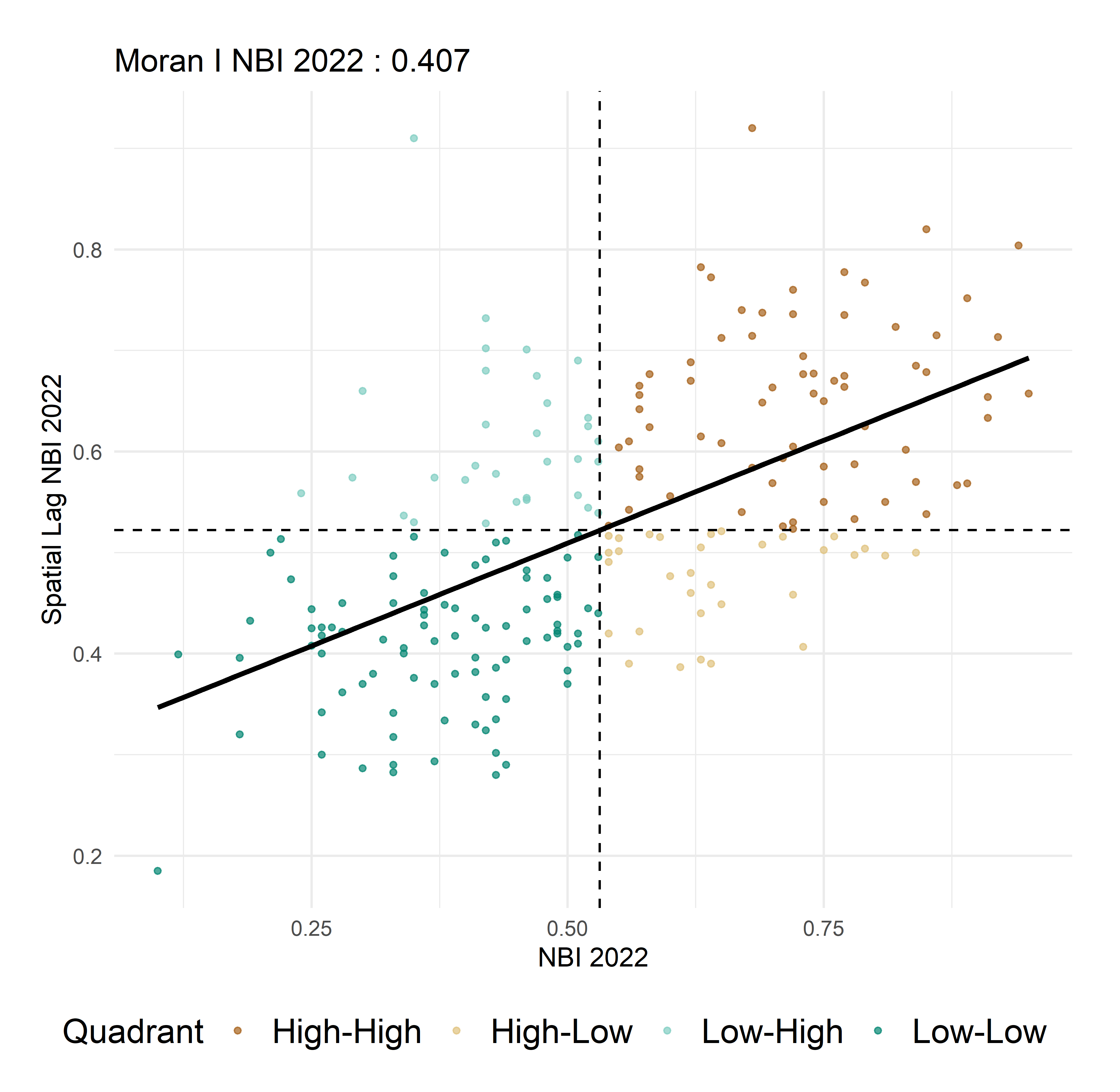
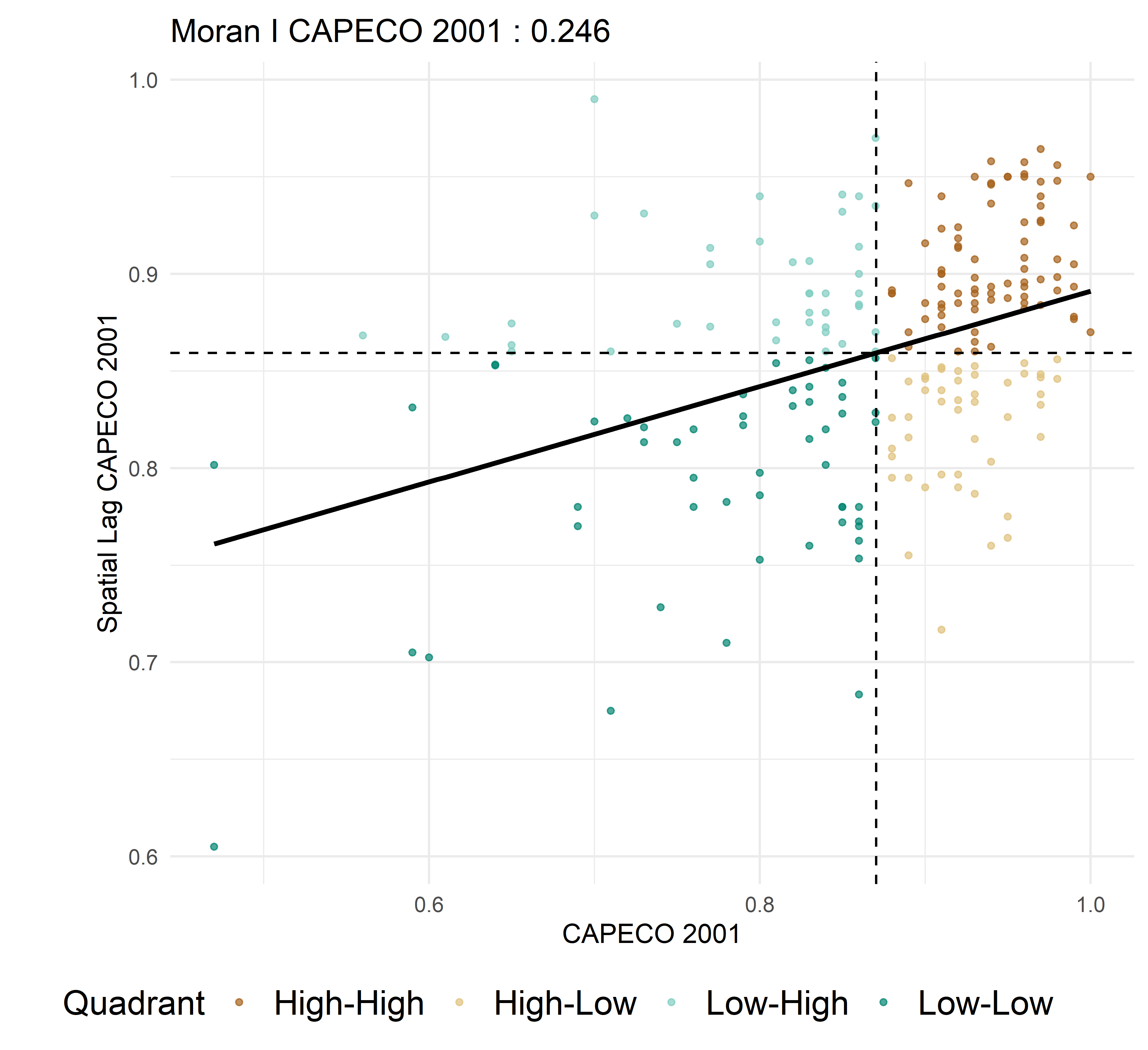
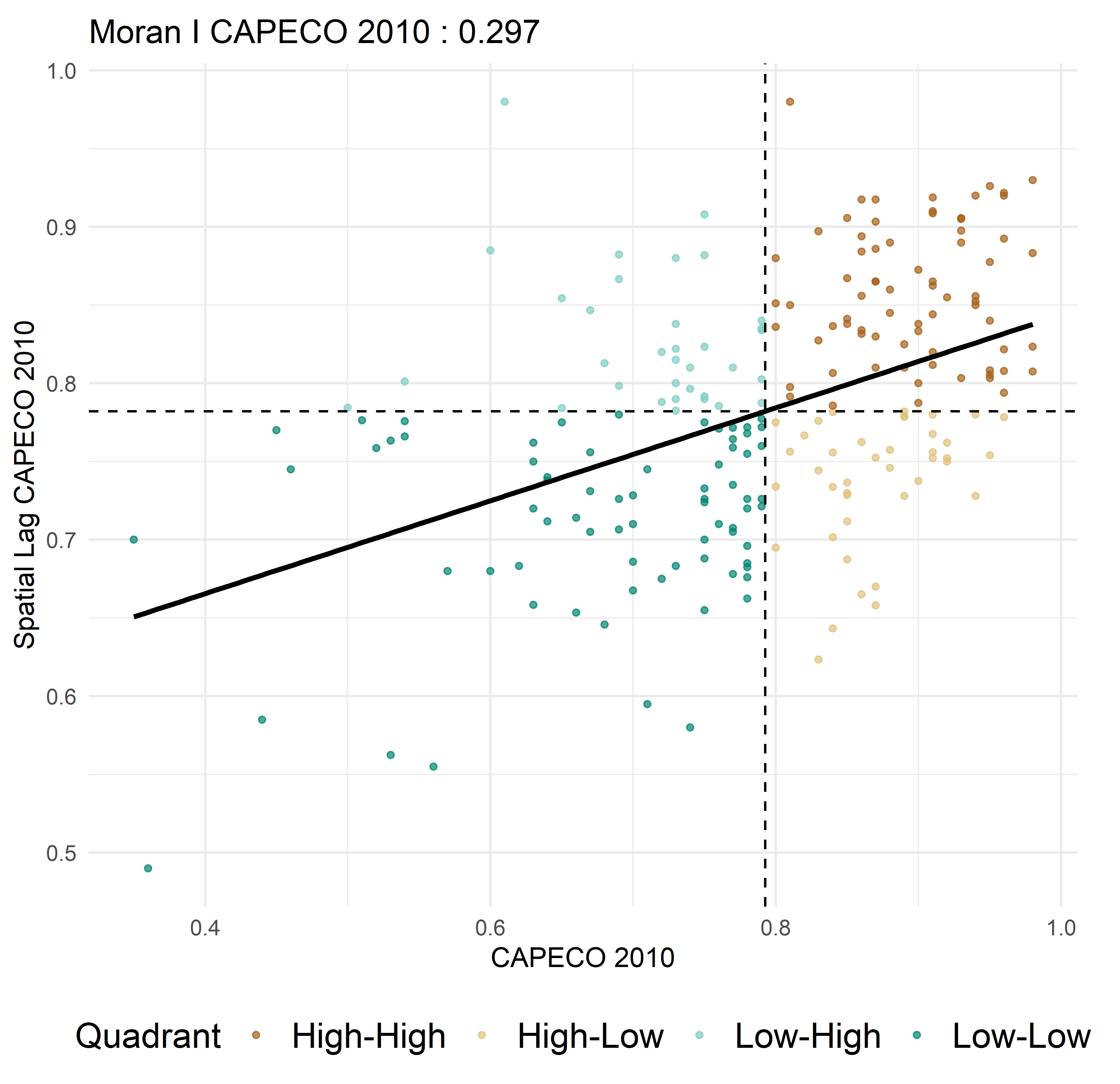
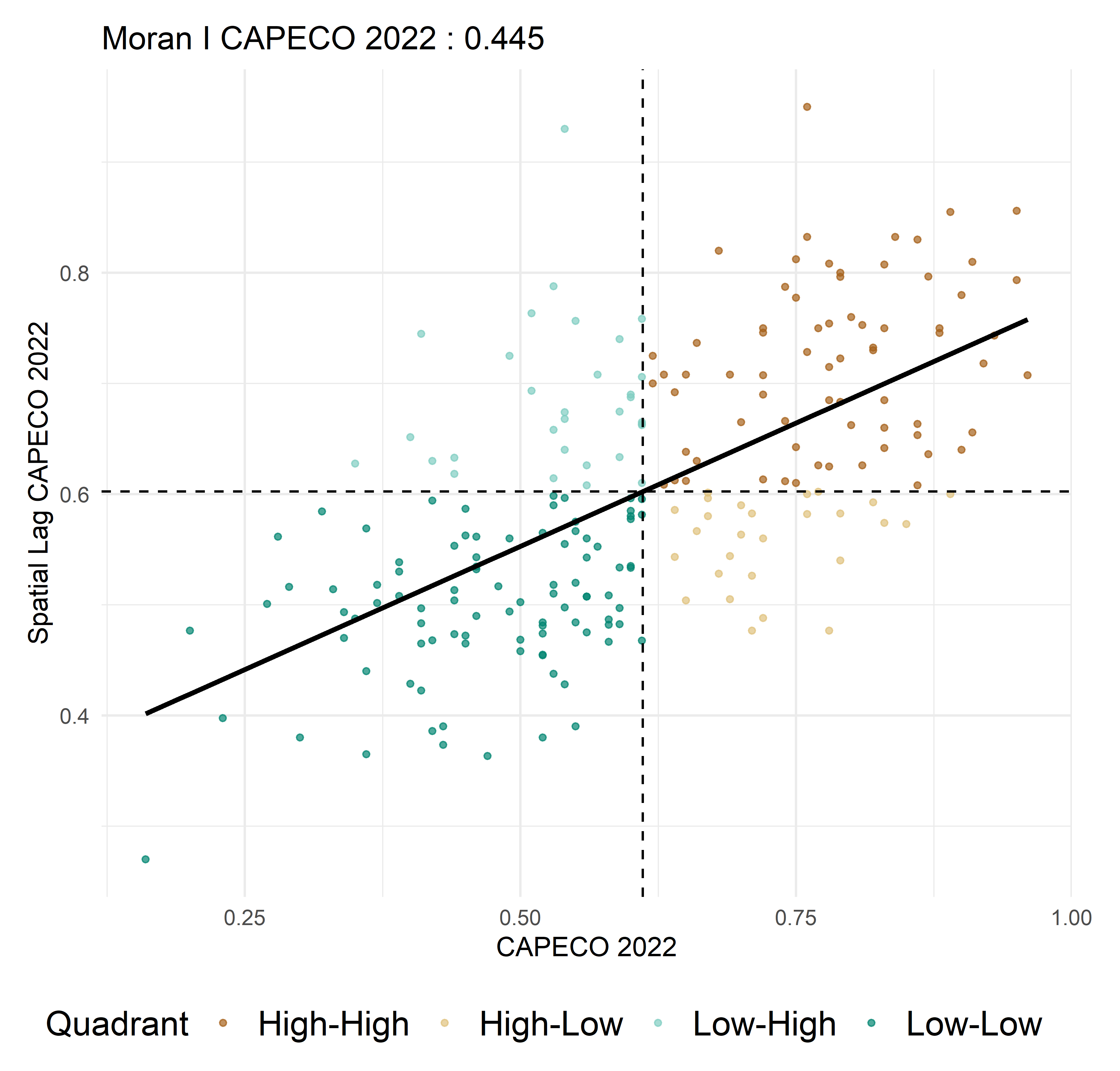
Figure 9 presents the evolution of Moran’s I for both the traditional UBN indicator and the CAPECO-modified measure. In 2001, the values of Moran’s I are positive and statistically significant, which indicates that cantons with similar levels of poverty tend to be geographically clustered rather than randomly distributed. This finding provides initial evidence of spatial dependence of poverty outcomes.
Over time, the magnitude of spatial autocorrelation increases substantially. As shown in figure 9, Moran’s I rises steadily between 2001 and 2022 for both indicators, which signals an intensification of spatial clustering. By 2022, the higher values of Moran’s I reflect a stronger tendency for high-poverty cantons to be surrounded by similarly deprived neighbors, and for low-poverty cantons to cluster together.
Source: Authors’ own elaboration.
This dynamic suggests a process of spatial polarization. Rather than converging, cantons appear to be increasingly grouped into homogeneous spatial regimes, characterized by either persistent deprivation or relative prosperity. The strengthening of spatial autocorrelation over time indicates that local conditions are becoming more closely aligned with those of neighboring territories, thereby reinforcing the role of geography as a determinant of poverty.
The corresponding Moran scatter plots further support this interpretation. The increasing concentration of observations in the high-high and low-low quadrants indicates that spatial clustering is driven primarily by the consolidation of homogeneous groups. In contrast, the relative scarcity of high-low and low-high observations suggests a decline in spatial heterogeneity, since fewer cantons deviate from the conditions of their surrounding areas (see Annex 1).
2.6 Local Moran’s I
While global Moran’s I provides an aggregate measure of spatial dependence, local indicators of spatial association (LISA) facilitate the identification of specific clusters and spatial outliers. Figure 10 presents the LISA cluster maps for the different years and highlights statistically significant patterns at the 5% level.
The results reveal a clear and persistent spatial structure. High-high clusters, defined as cantons with high poverty surrounded by similarly poor neighbors, are predominantly concentrated on the central and northern Coast. This pattern becomes more pronounced over time, with an expansion and consolidation of high-poverty clusters, particularly in provinces such as Manabí and Esmeraldas. These areas can be interpreted as territorial poverty traps, where structural disadvantages are reinforced by adverse spatial spillovers.
In contrast, low-low clusters are primarily located in the central-northern Sierra, where cantons with relatively low levels of poverty are surrounded by similarly advantaged neighbors. As shown in figure 10, these clusters remain relatively stable over time, with some expansion into adjacent territories which reflects gradual improvements in nearby areas.

Source: Authors’ own elaboration.
The evolution of local clusters suggests a process of spatial consolidation. High-poverty areas increasingly form contiguous blocks, while low-poverty regions reinforce their relative advantage. At the same time, the presence of spatial outliers (cantons classified as high-low or low-high) becomes less frequent, thereby indicating a reduction in transitional or mixed spatial configurations (see Annex 2).
Taken together, the evidence from figure 9 and figure 10 points to a strong and increasing degree of spatial dependence of poverty across Ecuador. Two key implications emerge.
First, poverty is not merely a local phenomenon but a spatially interconnected process, where outcomes in one canton are influenced by conditions in neighboring territories. This interdependence likely reflects shared labor markets, infrastructure networks, and productive linkages that transmit both advantages and disadvantages across space.
Second, the persistence and strengthening of spatial clusters indicate the emergence of territorially embedded poverty traps. High-poverty cantons are not isolated cases but form part of broader regional systems characterized by structural constraints that limit their capacity to converge towards more favorable conditions.
Overall, the spatial analysis demonstrates that poverty in Ecuador is increasingly organized along geographical lines, with clear patterns of clustering and polarization. These findings justify the use of spatial econometric models in the subsequent analysis, since ignoring spatial dependence would lead to biased estimates and an incomplete understanding of the mechanisms driving poverty dynamics.
3 Materials and Methods
3.1 Analysis of Factors Explaining Poverty and its Spatial Distribution
To identify the socioeconomic factors underlying poverty and its spatial dynamics, this study estimates a spatial panel data model using information for Ecuador’s 221 cantons over the years 2001, 2010, and 2022. The analysis considers two alternative measures of poverty (the traditional UBN indicator and the CAPECO-modified version) in order to assess the robustness of the results to differences in measurement.
3.2 Model Specification
Given the strong evidence of spatial dependence documented in the previous section, the empirical strategy adopts a spatial Durbin model (SDM) with two-way fixed effects. This specification enables the simultaneous modeling of spatial spillovers in both the dependent variable and the explanatory variables.
The empirical specification is expressed in matrix form for each period (\(t\)) as:
\[ \mathbf{y}_t = \rho \mathbf{W}\mathbf{y}_t + \mathbf{X}_t \boldsymbol{\beta} + \mathbf{W}\mathbf{X}_t \boldsymbol{\theta} + \boldsymbol{\alpha} + \gamma_t \mathbf{1}_N + \mathbf{u}_t \tag{2}\]
where \(\mathbf{y}_t\) is an \(N \times 1\) vector containing the poverty rate of the \(N\) cantons in period \(t\), \(\mathbf{W}\) is the \(N \times N\) spatial weights matrix, and \(\mathbf{W}\mathbf{y}_t\) denotes the spatial lag of the dependent variable. Thus, for each canton \(i\), the term \(\mathbf{W}\mathbf{y}_t\) represents a spatially weighted average of poverty rates in neighboring cantons. The matrix \(\mathbf{X}_t\) is an \(N \times K\) matrix of socioeconomic covariates, where each row corresponds to a canton and each column to a covariate. The term \(\mathbf{W}\mathbf{X}_t\) is therefore an \(N \times K\) matrix containing the spatially lagged covariates. The vectors \(\boldsymbol{\beta}\) and \(\boldsymbol{\theta}\) are \(K \times 1\) parameter vectors associated with local covariates and spatially lagged covariates, respectively. The vector \(\boldsymbol{\alpha}\) contains canton fixed effects, \(\gamma_t \mathbf{1}_N\) captures time fixed effects common to all cantons in period \(t\), and \(\mathbf{u}_t\) is an \(N \times 1\) vector of idiosyncratic error terms.
The inclusion of both spatial lags enables the model to capture direct effects (within-canton impacts) and indirect effects (spillovers across neighboring cantons), which are central to understanding the territorial dynamics of poverty.
3.3 Interpretation of coefficients
In the SDM framework, the estimated coefficients \(\beta\) and \(\theta\) do not directly correspond to marginal effects due to the presence of spatial feedback mechanisms. Instead, the total impact of each variable is decomposed into:
Direct effects, capturing the impact of changes within a canton.
Indirect effects, capturing spillovers to neighboring cantons.
Total effects, combining both components.
This decomposition is essential for correctly interpreting the role of each determinant in a spatial context. Following Elhorst (2014), and based on the estimation of the model’s structural parameters, the effects of the \(k\)-th regressor on \(\mathbf{y}_t\) are derived as follows:
\[ \mathbf{S}_k(\mathbf{W}) = (\mathbf{I}_N - \rho \mathbf{W})^{-1} (\beta_k \mathbf{I}_N + \theta_k \mathbf{W}) \]
\[ \text{Direct effect} = \overline{\operatorname{diag}[\mathbf{S}_k(\mathbf{W})]} \]
\[ \text{Total effect} = \overline{\operatorname{rsum}[\mathbf{S}_k(\mathbf{W})]} \]
\[ \text{Indirect effect} = \overline{\operatorname{rsum}[\mathbf{S}_k(\mathbf{W})]} - \overline{\operatorname{diag}[\mathbf{S}_k(\mathbf{W})]} \]
where \(\mathbf{S}_k(\mathbf{W})\) is the \(N \times N\) matrix of partial derivatives associated with the \(k\)-th explanatory variable, \(\mathbf{I}_N\) is the \(N \times N\) identity matrix, \(\rho\) is the spatial autoregressive parameter, \(\beta_k\) is the coefficient of the local covariate, and \(\theta_k\) is the coefficient of its spatial lag. The statistical significance of the direct, indirect, and total effects was assessed using a parametric bootstrap procedure. A total of 5,000 simulated samples of the coefficients were generated from their variance-covariance matrix, and spatial effects were recalculated in each simulation. Confidence intervals at 90%, 95%, and 99% were constructed, and an effect was considered significant if its interval excluded zero, following the methodology recommended for spatial models with complex dependencies (Jin & Lee, 2013).
3.4 Model Selection and Estimation
The selection of the spatial specification follows a Bayesian model comparison framework as proposed by LeSage (2014), which provides a coherent and simultaneous evaluation of alternative spatial models. Recent studies have adopted this approach (Herrera, 2021; Li et al., 2025; Pommeranz & Steininger, 2020; Saucedo de la Fuente & Berry, 2019; Yesilyurt & Elhorst, 2017). In contrast to conventional approaches based on sequential hypothesis testing, such as the likelihood ratio and Wald tests, this method assesses the relative plausibility of competing specifications by comparing their posterior model probabilities.
Formally, let \(\mathcal{M}_{k}\) denote a set of candidate models, including the spatial autoregressive model (SAR), the spatial Durbin model (SDM), the spatial error model (SEM), the dpatial Durbin error model (SDEM), and the spatially lagged X model (SLX). Prior probabilities are assigned uniformly across models, which reflect the absence of prior preference:
\[P\left( \mathcal{M}_{k} \right) = \frac{1}{K},\ \ \forall\ k \tag{3}\]
For each model, the marginal likelihood of the data is computed as:
\[P\left( y \middle| \mathcal{M}_{k} \right) = \int_{}^{}{P\left( y \middle| \theta_{k},\ \mathcal{M}_{k} \right)P\left( \theta_{k} \middle| \mathcal{M}_{k} \right)d\theta_{k}} \tag{4}\]
where \(P\left( y \middle| \theta_{k},\ \mathcal{M}_{k} \right)\) is the likelihood function and \(P\left( \theta_{k} \middle| \mathcal{M}_{k} \right)\) denotes the prior distribution of the parameters. This integration accounts for parameter uncertainty and penalises model complexity in a natural way. Posterior model probabilities are then obtained via Bayes’ rule:
\[P\left( \mathcal{M}_{k} \middle| y \right)\ = \ \frac{P\left( y \middle| \ \mathcal{M}_{k} \right)P(\mathcal{M}_{k})}{\sum_{j = 1}^{K}{P\left( y \middle| \ \mathcal{M}_{j} \right)P(\mathcal{M}_{j})}} \tag{5}\]
These probabilities provide a direct ranking of competing specifications, thereby yielding the identification of the model that best balances goodness-of-fit and parsimony. The empirical results indicate that the spatial Durbin model (SDM) exhibits the highest posterior probability (see Annex 3) , since it clearly outperforms alternative specifications. This finding suggests that spatial dependence operates not only through the dependent variable but also through the explanatory variables, there by supporting the presence of indirect transmission mechanisms across cantons. A major advantage of this approach is that it facilitate the comparison of both nested and non-nested models within a unified probabilistic framework, while avoiding the path-dependence and potential inconsistencies associated with sequential testing procedures. Moreover, by integrating over the parameter space, the method takes estimation uncertainty into account, which leads to a more robust model selection.
4 Results and Limitations
According to table 6, Ecuador underwent substantial demographic, social, and economic transformations between 2001 and 2022. Average household size declined from 4.38 to 3.28 members due to ongoing urbanization processes and changes in family structures. The population aged moderately, as the share of older adults increased, while the proportion of young individuals remained broadly stable. At the same time, female-headed households rose markedly, from 23.82% to 36.57%, which indicated shifts in household composition and in gender roles. The proportion of individuals self-identifying as indigenous increased slightly, whereas the share of Afro-Ecuadorians exhibited no clear trend. Population density also increased significantly, from 87.78 to 124.49 inhabitants per km², consistent with rising urban concentration.
From an economic perspective, the period was characterized by a process of structural transformation. The share of employment in the primary sector declined sharply, from 53.07% to 37.51%, while the tertiary sector expanded substantially, from 29.80% to 51.75%. The secondary sector remained relatively stable. Informal employment decreased considerably, and emigration rates fell, suggesting improvements in local labor market conditions and reduced incentives to migrate.
Despite these advances, major structural challenges persist. Pension coverage remains limited, with only 3.31% of older adults receiving retirement income in 2022, pointing to gaps in social protection systems. More critically, the unemployment rate increased dramatically from 1.79% to 20.37%, thereby revealing a significant deterioration in labor market performance. This trend, coupled with marked regional disparities, suggests that the observed structural transformation has not been accompanied by sufficient job creation, which has limited its capacity to reduce poverty in a sustained and inclusive manner.
Source: Authors’ own elaboration.
4.1 Spatial Model Estimation
Table 7 reports the estimation results of the spatial Durbin model (SDM) for both poverty measures. The reported coefficients correspond to the structural parameters of the model, including the effects of the explanatory variables and their spatial lags, as well as the spatial autoregressive parameter.
At the outset, it is important to emphasize that the estimated coefficients associated with the explanatory variables and their spatial lags do not represent marginal effects in the conventional sense. Due to the presence of spatial feedback mechanisms, changes in one canton propagate through the spatial system and may return to the original unit. As a result, these coefficients capture only the initial impact of each variable, prior to the full adjustment process. For this reason, they are not directly interpretable in isolation and must be analyzed through the decomposition into direct, indirect, and total effects presented in the following section.
A key result concerns the spatial autoregressive parameter (\(\mathbf{\lambda}\)), which is positive and highly statistically significant across all specifications. The estimated magnitude, of approximately 0.77, indicates a strong degree of spatial dependence in poverty outcomes. This implies that poverty levels in a given canton are closely linked to those observed in neighboring cantons, reflecting the presence of spatial spillovers. Such interdependence is consistent with mechanisms such as shared labour markets, interregional mobility, local production linkages, and coordinated or overlapping policy environments.
The strength of the spatial parameter suggests that poverty in Ecuador is not an isolated local phenomenon but rather a territorially interconnected process. Consequently, shocks affecting one canton, whether they be economic, demographic, or institutional, are likely to propagate across space, reinforcing regional patterns of deprivation or improvement.
The goodness-of-fit of the model, as captured by the pseudo-\(R^{2}\), is high in all specifications, exceeding 0.96. Following Elhorst (2014), this measure reflects the explanatory power of the full spatial model, including the contribution of spatial lags and fixed effects. Therefore, its magnitude should not be interpreted as evidence of the explanatory capacity of the regressors alone, but rather as an indication that the combined structure of spatial dependence and unobserved heterogeneity captures a substantial share of the variation in poverty across cantons and over time.
Overall, the estimation results confirm the presence of strong spatial interdependence and provide a consistent empirical foundation for the analysis of the determinants of poverty. The subsequent section builds on these findings by decomposing the effects of the explanatory variables into direct and indirect components, thereby facilitating a more precise interpretation of the mechanisms through which poverty is generated and transmitted across space.
| Variable | CAPECO UBN | Traditional UBN | CAPECO UBN | Traditional UBN |
|---|---|---|---|---|
| Human capital | -0.2512*** (0.0278) |
-0.2836*** (0.0336) |
0.0977*** (0.0372) |
0.1138** (0.0469) |
| Household size | 0.1139** (0.0514) |
0.1305** (0.0623) |
-0.2836*** (0.0706) |
-0.2986*** (0.0846) |
| Older adult population | 0.6216*** (0.1734) |
0.7355*** (0.2102) |
-1.1762*** (0.2166) |
-1.3545*** (0.2629) |
| Youth population | 1.5727*** (0.2079) |
1.8023*** (0.2524) |
-1.4865*** (0.3711) |
-1.7284*** (0.4555) |
| Female-headed households | -0.0079 (0.0743) |
-0.0946 (0.0903) |
-0.3322*** (0.1091) |
-0.2977** (0.1353) |
| Indigenous population | 0.0901*** (0.0248) |
0.1208*** (0.0302) |
-0.1156*** (0.0361) |
-0.1409*** (0.0439) |
| Afro-Ecuadorian population | 0.2277*** (0.0642) |
0.3007*** (0.0781) |
-0.3483*** (0.0899) |
-0.4455*** (0.1092) |
| Population density | -0.0107*** (0.0039) |
-0.0118* (0.0047) |
0.0008 (0.0062) |
0.0027 (0.0075) |
| Primary sector | 0.0790*** (0.0188) |
0.0914*** (0.0229) |
-0.0461 (0.0344) |
-0.0508 (0.0418) |
| Secondary sector | 0.0988* (0.0520) |
0.1216* (0.0636) |
-0.1468* (0.0864) |
-0.2051* (0.1050) |
| Tertiary sector | -0.2750*** (0.0399) |
-0.2872*** (0.0484) |
0.2893*** (0.0762) |
0.3427*** (0.0893) |
| Emigration | 0.1648* (0.0872) |
0.1722 (0.1059) |
-0.0578 (0.1223) |
-0.0448 (0.1490) |
| Unemployment rate | 0.4779*** (0.0750) |
0.3692*** (0.0911) |
-0.1466 (0.1484) |
-0.0206 (0.1766) |
| Retirement income | -0.1845* (0.1048) |
-0.2157* (0.1271) |
0.4339** (0.1765) |
0.4298** (0.2109) |
| Informal employment rate | -0.0958** (0.0456) |
-0.1126** (0.0408) |
0.1345* (0.0745) |
0.1599* (0.0905) |
| Lambda (λ) | 0.7708*** | 0.7768*** | ||
| Pseudo R^2 | 0.9637 | 0.9603 |
Source: Authors’ own elaboration.
Note: *** significant at 1%, ** significant at 5%, * significant at 10%.
4.2 Spatial Effects of Explanatory Factors on Regional Poverty
In the context of the spatial Durbin model (SDM), the presence of spatial feedback effects implies that the impact of explanatory variables extends beyond the location of the shock. A change in a given canton not only affects local poverty levels but also propagates through neighboring units and feeds back into the original location. As a result, the total impact of each variable must be evaluated in terms of its long-term effects.
Following Elhorst (2014), the effects of a change in an explanatory variable are decomposed into three components. The direct effect captures the average impact of a change within a canton on its own poverty level, including the influence of feedback loops. The indirect effect (or spillover effect) reflects the impact transmitted to neighboring cantons through the spatial structure. The total effect corresponds to the sum of the two components and represents the overall impact on the system.
Table 8 reports the estimated direct, indirect, and total effects for each explanatory variable. Statistical significance is assessed using a parametric bootstrap procedure with 5000 simulations, which accounts for the complex dependence structure of the model. Confidence intervals are constructed at conventional levels, and an effect is considered statistically significant when its interval does not include zero (Jin & Lee, 2013).
| Variable | CAPECO UBN | Traditional UBN | CAPECO UBN | Traditional UBN | CAPECO UBN | Traditional UBN |
|---|---|---|---|---|---|---|
| Human capital | -0.277*** | -0.313*** | -0.387*** | -0.441** | -0.664*** | -0.754** |
| Household size | 0.061 | 0.076 | -0.790*** | -0.817** | -0.729** | -0.741* |
| Older adult population | 0.433** | 0.519** | -2.812*** | -3.245** | -2.379*** | -2.726** |
| Youth population | 1.499*** | 1.712*** | -1.106 | -1.360 | 0.393 | 0.351 |
| Female-headed households | -0.099 | -0.197** | -1.365*** | -1.538** | -1.464*** | -1.735** |
| Indigenous population | 0.078*** | 0.108*** | -0.186 | -0.195 | -0.109 | -0.087 |
| Afro-Ecuadorian population | 0.181*** | 0.239*** | -0.697*** | -0.919** | -0.516** | -0.679** |
| Population density | -0.013*** | -0.014*** | -0.030 | -0.027 | -0.043** | -0.041 |
| Primary sector | 0.083*** | 0.096*** | 0.059 | 0.084 | 0.143 | 0.181 |
| Secondary sector | 0.079 | 0.091 | -0.285 | -0.459 | -0.205 | -0.368 |
| Tertiary sector | -0.254*** | -0.254*** | 0.312 | 0.496 | 0.058 | 0.241 |
| Emigration | 0.183** | 0.197* | 0.279 | 0.369 | 0.463 | 0.565 |
| Unemployment rate | 0.538*** | 0.442*** | 0.895* | 1.103* | 1.433** | 1.546** |
| Retirement income | -0.106 | -0.143 | 1.177* | 1.087 | 1.071 | 0.943 |
| Informal employment rate | -0.079 | -0.092 | 0.244 | 0.300 | 0.165 | 0.208 |
Source: Authors’ own elaboration.
Note: *** significant at 1%, ** significant at 5%, * significant at 10%.
4.3 Human Capital
Human capital, measured as the average years of schooling among individuals aged 25 and above, emerges as the most robust determinant of poverty reduction. The direct effects are negative and statistically significant, and indicate that higher educational attainment reduces poverty within cantons.
The indirect effects are also negative and significant, revealing the presence of positive spatial spillovers. This suggests that improvements in education generate benefits beyond local boundaries, probably through labor mobility and knowledge diffusion. As a result, the total effects are substantial, thereby highlighting the system-wide impact of human capital.
These findings are consistent with human capital theory (Becker, 1994) and with evidence on the social returns from education (Psacharopoulos & Patrinos, 2018). Furthermore, results remain robust across both poverty measures, which indicates that education influences poverty through multiple channels beyond its direct inclusion in the CAPECO indicator. Overall, human capital constitutes a central mechanism for the reduction of poverty and mitigation of spatial disparities, with effects that extend across neighboring territories.
4.4 Productive structure
The productive structure exhibits differentiated effects on poverty. A higher concentration of employment in the primary sector is associated with increased poverty due to its low productivity and limited income-generating capacity (Ravallion & Datt, 1996). In contrast, the tertiary sector shows a negative and significant direct effect, which indicates that service-based activities contribute to poverty reduction. Indirect effects are generally not statistically significant, which suggests that the impact of productive structure is predominantly local. Overall, these findings support the role of structural transformation towards higher value-added activities as a key pathway for the reduction of poverty (World Bank, 2009).
4.5 Sociodemographic characteristics
Sociodemographic factors exhibit heterogeneous and spatially differentiated effects on poverty. The proportion of young people in the population is positively associated with poverty at the local level, due to constraints in labor market entry and the limited absorption capacity of local economies. This result is consistent with evidence on youth unemployment and precarious employment in developing contexts, where weak school-to-work transitions increase vulnerability (International Labour Organization, 2019). The absence of statistically significant spillover effects suggests that these constraints are largely localized and depend on the specific labor market conditions of each canton.
In contrast, the proportion of older adults shows a more complex pattern. While the direct effects are positive in that ageing increases dependency ratios and reduces labor income at the local level, the indirect effects are negative and statistically significant. This suggests that ageing may generate beneficial spillovers in neighboring cantons, potentially through mechanisms such as inter-household transfers, pension income redistribution, and increased demand for health and care services (Inter-American Development Bank, 2018). These findings highlight the dual role of demographic ageing as both a source of vulnerability and a channel of regional economic interaction.
Female-headed households are associated with reductions in poverty, particularly through spillover effects. While the direct effects are modest, the indirect and total effects are negative and statistically significant, which indicates that their impact extends beyond local boundaries. This result challenges traditional assumptions that link female headship exclusively to higher vulnerability. Instead, it is consistent with evidence that suggests that female-headed households often allocate resources more efficiently towards education, health, and housing, and may benefit from remittance flows that improve household welfare (Liu et al., 2017; World Bank, 2020). The presence of spatial spillovers further suggests that these effects may contribute to broader regional improvements.
Overall, sociodemographic characteristics shape poverty dynamics through multiple and interacting channels. While certain effects are primarily local, such as those associated with youth, others generate significant spatial spillovers, particularly in the case of ageing and female headship. These patterns underscore the importance not only of incorporating demographic structure into the analysis of poverty, but also of designing policies that account for both local conditions and interregional linkages.
4.6 Emigration
With respect to the proportion of households with a permanent migrant, the direct effect is 0.183 (p < 0.05) in CAPECO and 0.197 (p < 0.10) in UBN, while both indirect and total effects are positive but not statistically significant. The positive local association suggests that emigration is not associated with lower poverty, potentially since remittances are not invested in structural improvements or because the departure of active household members reduces productive capacity (Ekanayake & Moslares, 2020; World Bank, 2018). The literature on remittances and poverty in LAC reports mixed effects: their impact depends on expenditure patterns and allocation. These findings highlight the need to examine remittance use in Ecuador and to support policies that channel funds toward productive investment and household infrastructure (World Bank, 2018).
4.7 Labor Market Characteristics
Labor market conditions emerge as a central determinant of poverty and its spatial propagation. The unemployment rate exhibits large and statistically significant direct and total effects that indicate that increases in unemployment substantially raise poverty at the local level. This finding reflects the critical role of labor income in sustaining household welfare, since the absence of employment directly constrains income generation and increases vulnerability. Moreover, the presence of positive and significant indirect effects suggests that unemployment shocks are not confined to individual cantons but propagate across neighboring territories, thereby reinforcing regional disparities. This spatial transmission is consistent with shared labor markets, commuting patterns, and interlinked local economies (International Labour Organization, 2019).
The magnitude of the total effects highlights unemployment as one of the most influential factors in shaping poverty dynamics within the model. From a structural perspective, this result points to weaknesses in labor market absorption capacity and the limited ability of local economies to generate stable employment opportunities. The sharp increase in unemployment observed over the period under study further reinforces its role as a key driver of persistent deprivation.
By contrast, the effects of informal employment are not statistically robust. While the direct effects are negative, which suggests that informality may provide short-term income and partially mitigate poverty at the local level, the indirect effects are positive, which indicates potential adverse spillovers across neighboring cantons. Although these estimates lack statistical significance, their signs are economically meaningful and reflect the dual nature of informality. On the one hand, informal employment can act as a coping mechanism in the context of limited formal job opportunities, by providing subsistence income and reducing immediate poverty (Loayza, 2018; Maloney, 2004). On the other hand, its expansion may generate negative externalities, such as increased competition in low-productivity sectors, erosion of formal labor markets, and a reduced fiscal base for public investment (Organisation for Economic Co-operation and Development, 2018).
Overall, the results indicate that labor market conditions play a pivotal role in both the local generation and spatial transmission of poverty. In particular, unemployment operates as a key mechanism through which economic shocks translate into persistent and geographically concentrated deprivation. These findings underscore the importance of policies aimed at strengthening labor market performance, including job creation, the development of skills, and coordinated regional employment strategies.
5 Conclusions and Discussion
This paper examines the spatial and temporal dynamics of poverty in Ecuador at the cantonal level between 2001 and 2022, by combining an extended UBN framework with the CAPECO index and a spatial econometric approach. The results provide consistent evidence that, although poverty has declined substantially over time, this has been an uneven process characterized by persistent territorial disparities.
First, the analysis shows that improvements in poverty have been dimension-specific. While notable progress has been achieved in housing conditions, overcrowding, and school attendance, access to basic services and household economic capacity remain the most critical constraints. These persistent deficits indicate that structural poverty in Ecuador is closely linked to infrastructural gaps and limited income-generating capacity, which have not been fully addressed by aggregate economic growth.
Second, the spatial analysis reveals an increasing degree of geographical concentration. Both global and local measures of spatial autocorrelation indicate a strengthening of high-high poverty clusters along the central and northern Coast, particularly in provinces such as Manabí and Esmeraldas, alongside the consolidation of low-low clusters in the central-northern Sierra. This pattern reflects a process of spatial polarization, where cantons increasingly resemble their neighbors, thereby reinforcing the territorial nature of poverty and limiting convergence across regions.
Third, the distributional analysis indicates that poverty reduction has been accompanied by limited mobility across cantons. The persistence observed at both ends of the distribution suggests the presence of convergence clubs and territorial poverty traps, where initial conditions continue to shape long-term outcomes. These findings highlight that, despite overall progress, structural barriers prevent lagging territories from catching up.
Fourth, the econometric results identify the key mechanisms underlying these dynamics. Human capital emerges as the most robust factor for the reduction of poverty, by generating both local improvements and positive spatial spillovers. In contrast, unemployment stands out as the main driver of poverty and its spatial propagation, and reflects structural weaknesses in labor markets. The productive structure also plays a major role, with dependence on the primary sector associated with higher poverty, while the expansion of the tertiary sector contributes to its reduction.
Additional findings point to the importance of sociodemographic and structural factors. Female-headed households are associated with reductions in poverty, particularly through spillover effects, while demographic composition, especially in the form of the presence of youth and older adults, affects poverty through distinct local and spatial channels. Furthermore, the persistent association between poverty and ethnic composition underscores the role of historical and structural inequalities in shaping territorial disparities.
Taken together, these results indicate that poverty in Ecuador is a multidimensional and spatially interdependent phenomenon. Its persistence is not only driven by local conditions but also reinforced by spatial interactions across cantons. As a result, policies that focus exclusively on individual territories may be insufficient to generate sustained and inclusive reductions in poverty.
From a policy perspective, the findings suggest three main priorities. First, targeted investments in basic services should be directed towards high-poverty clusters, particularly in the Coastal region, to address persistent infrastructural deficits. Second, labor market policies should prioritize employment generation, especially for youth, and strengthen regional coordination in order to mitigate the spatial transmission of unemployment shocks. Third, education policy should focus not only on expanding coverage but also on improving quality and aligning skills with local economic structures, in order to maximize both local and spillover effects.
In conclusion, while Ecuador has achieved significant progress in reducing poverty, the persistence of territorial inequalities and the strengthening of spatial clustering indicate that structural challenges remain. Overcoming these constraints will require a shift towards integrated, location-based development strategies that both bear spatial interdependence in mind and target the underlying drivers of regional inequality.
Annexes
Annex 1. Cantons with High-High Clusters According to Local Moran’s I (2001, 2010, and 2022)
| 2001 | 2010 | 2022 | Province |
|---|---|---|---|
| Balzar, Colimes, Pedro Carbo, Santa Lucía | Balzar, Colimes, Pedro Carbo, Santa Lucía, Palestina | Balzar, Colimes, Pedro Carbo, Santa Lucía, Palestina, El Empalme | Guayas |
| Paján | Paján, Chone, Jipijapa, 24 de Mayo, Olmedo | Paján, Chone, Jipijapa, 24 de Mayo, Olmedo, Pichincha, Santa Ana, Tosagua, Pedernales, Jama | Manabí |
| Lago Agrio | Sucumbíos | ||
| Pallatanga | Pallatanga | Chimborazo | |
| Quinindé | Quinindé, Eloy Alfaro, Atacames | Esmeraldas | |
| Vinces | Vinces, Mocache | Los Ríos |
Annex 2. Cantons with Low-Low Clusters According to Local Moran’s I (2001, 2010, and 2022)
| 2001 | 2010 | 2022 | Province |
|---|---|---|---|
| Mira | Mira | Bolívar | Carchi |
| Rumiñahui, Distrito Metropolitano de Quito, Cayambe, Mejía, Pedro Moncayo | Rumiñahui, Distrito Metropolitano de Quito, Cayambe, Mejía, Pedro Moncayo | Rumiñahui, Distrito Metropolitano de Quito, Cayambe, Pedro Moncayo | Pichincha |
| Antonio Ante, Otavalo | Otavalo, San Miguel de Urcuquí | Otavalo | Imbabura |
| Santa Rosa | Santa Rosa | Santa Rosa, Arenillas, Piñas | El Oro |
| Paute, San Fernando | Paute, San Fernando, Cuenca, Gualaceo, Sevilla de Oro, Guachapala | Azuay | |
| Biblián, Déleg | Cañar | ||
| San Pedro de Pelileo, Tisaleo | Tungurahua | ||
| Durán | Balao | Guayas |
Annex 3. Model Variables
| Variable | Description |
|---|---|
| Dependent Variable: | |
| Poverty Rate in terms of UBNs | The percentage of total households in the canton lacking at least one basic need. |
| Independent Variables: | |
| Population density | Number of inhabitants per square kilometer |
| Household size | Average number of members per household |
| Older Adult Population | Percentage of people over 65 years old |
| Youth Population | Percentage of people between 15 and 25 years old |
| Female-headed households | Percentage of households headed by a woman |
| Emigration | Percentage of households with at least one member who has emigrated permanently |
| Human capital | Average years of schooling among people over 24 years old |
| Labor concentration in the primary, secondary, or tertiary sectors | Percentage of the total workforce in each sector |
| Informal employment rate | Percentage of workers who are self-employed or salaried without affiliation to IESS |
| Indigenous population | Percentage of the total population that self-identifies as indigenous |
| Retirement Income | Percentage of older adults who receive a pension |
| Unemployment Rate | Percentage of people not working and actively seeking employment |
| Afro-Ecuadorian population | Percentage of the population that self-identifies as Afro-Ecuadorian |
Annex 4. Lesage’s Bayesian Test for Two-Way Fixed Effects
| OLS | SAR | SDM | SEM | SDEM | SLX | |
|---|---|---|---|---|---|---|
| Log marginals | 613.766 | 637.652 | 637.906 | 629.129 | 637.716 | 630.651 |
| Model probs | 0.000 | 0.2980 | 0.3839 | 0.0001 | 0.3177 | 0.0003 |
References
Acevedo González, K., Quejada Pérez, R., & Yánez Contreras, M. (2010). Determinantes y consecuencias del trabajo infantil: Un análisis de la literatura. Revista Facultad de Ciencias Económicas, 19(1), 113–124. https://doi.org/10.18359/rfce.2263
Acuña Carrasco, J. A., Castro Balderrama, C. A., & Mansilla Bustamante, S. A. (2017). Análisis espacial de la persistencia de pobreza a nivel municipal. Sociedad Científica Estudiantil de Economía (SCEE), (3), 47–66.
Álvarez, G. (2002). Capacidad económica de los hogares. Una aproximación a la insuficiencia de ingresos. Notas de Población, 29(74), 213–250.
Aponte, C., Romero, E., & Santa, L. (2015). Análisis de datos espaciales del índice de necesidades básicas insatisfechas en la región andina. Perspectiva Geográfica, 20(2), 391–418. https://doi.org/10.19053/01233769.4533
Becker, G. S. (1994). Human capital: A theoretical and empirical analysis, with special reference to education (3rd ed.). National Bureau of Economic Research. https://econpapers.repec.org/bookchap/nbrnberbk/beck94-1.htm
Bradshaw, T. K. (2007). Theories of poverty and anti-poverty programs in community development. Community Development, 38(1), 7–25. https://doi.org/10.1080/15575330709490182
Economic Commission for Latin America and the Caribbean. (2015). Guía metodológica instrumentos económicos para la gestión ambiental. https://repositorio.cepal.org/server/api/core/bitstreams/3c220f39-febd-49ae-ad82-8bec29caa14f/content
Ekanayake, E. M., & Moslares, C. (2020). Do remittances promote economic growth and reduce poverty? Evidence from Latin American countries. Economies, 8(2), 35. https://doi.org/10.3390/economies8020035
Elhorst, J. P. (2014). Spatial econometrics: From cross-sectional data to spatial panels. Springer Berlin Heidelberg. https://doi.org/10.1007/978-3-642-40340-8
García Vélez, D. F., & Núñez Velázquez, J. J. (2022). Un enfoque alternativo para medir la pobreza multidimensional utilizando conjuntos difusos: Análisis espacial para Ecuador. Investigaciones Regionales - Journal of Regional Research, 52, 37–58. https://doi.org/10.38191/iirr-jorr.22.002
Gigler, B. S. (2015). Development as freedom in a digital age: Experiences from the rural poor in Bolivia. The World Bank. http://elibrary.worldbank.org/doi/book/10.1596/978-1-4648-0420-5
Gómez, A., Álvarez, G., Olmos, F., & Lucarini, A. (1999). Capacidad económica de los hogares. Vinculaciones entre la pobreza coyuntural y los comportamientos demográficos. Provincias seleccionadas, 1991. V Jornadas Argentinas de Estudios de La Población. https://www.aacademica.org/gustavo.oscar.alvarez/23.pdf
Herrera, C. J. R. A. (2021). Impacto de las remesas en la pobreza y en la oferta laboral del Ecuador. Un estudio desde la perspectiva económica y demográfica. Revista Visión Contable Universidad Autónoma Latinoamericana, (24), 101–126.
Instituto Nacional de Estadística y Censos. (2024a). Censo población y vivienda. https://www.ecuadorencifras.gob.ec/pobreza-por-necesidades-basicas-insatisfechas/
Instituto Nacional de Estadística y Censos. (2024b). Ficha metodológica por indicador. https://www.censoecuador.gob.ec/wp-content/uploads/2024/04/Porcentaje_de_personas_u_hogares_en_Pobreza_por_NBI.pdf
Inter-American Development Bank. (2018). Presente y futuro de las pensiones en América Latina y el Caribe. https://www.fiapinternacional.org/en/the-present-and-future-of-pensions-in-latin-america-and-the-caribbean-idb-november-2018/
International Labour Organization. (2019). World employment and social outlook: Trends 2019. http://ilo.org/sites/default/files/wcmsp5/groups/public/%40dgreports/%40dcomm/%40publ/documents/publication/wcms_670542.pdf
Jin, F., & Lee, L. (2013). On the bootstrap for spatial econometric models. https://econ.sufe.edu.cn/_upload/article/files/94/e5/ae50286b4f7a91fcbae94f07c82b/26cd428f-751a-4e07-a1c6-b5fa904664d4.pdf
Jung, H.-S., & Thorbecke, E. (2003). The impact of public education expenditure on human capital, growth, and poverty in tanzania and zambia: A general equilibrium approach. Journal of Policy Modeling, 25(8), 701–725.
LeSage, J. P. (2014). Spatial econometric panel data model specification: A bayesian approach. Spatial Statistics, 9, 122–145. https://doi.org/10.1016/j.spasta.2014.02.002
Levernier, W., Partridge, M. D., & Rickman, D. S. (2000). The causes of regional variations in u.s. Poverty: A cross-county analysis. Journal of Regional Science, 40(3), 473–497. https://doi.org/10.1111/0022-4146.00184
Li, J., Hu, Y., Wang, N., Wang, S. suspicion, Wang, R., Lyu, L., & Fang, Z. (2025). Advances and trends in Bayesian spatio-temporal statistical methods and applications. Journal of Geo-Information Science, 27(7), 1501–1519. https://doi.org/10.12082/dqxxkx.2025.250161
Liu, C., Esteve, A., & Treviño, R. (2017). Female-headed households and living conditions in Latin America. World Development, 90(C), 311–328.
Loayza, N. (2018). Informality: Why is it so widespread and how can it be reduced? https://papers.ssrn.com/abstract=3360124
López Ávila, D. M. (2009). Pobreza y trabajo infantil: Diferencias entre trabajo dentro y fuera del hogar. Evidencia para Colombia, 2001-2003 [Documentos de Econom{\'\i}a]. (No. 7754). https://ideas.repec.org/p/col/000108/007754.html
López-Calva, L. F. (2006). Trabajo infantil: Teorı́a y lecciones de la América Latina. Fondo de Cultura Económica.
Maloney, W. F. (2004). Informality revisited. World Development, 32(7), 1159–1178.
Mario, S., Gómez, A., & Martins Pereira, N. de O. (2004). Aplicación del indicador de capacidad económica de los hogares (CAPECO) en el marco del proyecto del censo común del MERCOSUR + 2 (Bolivia y Chile). https://files.alapop.org/alap/images/PDF/ALAP2004_267.pdf
Noceti, M. B. (2011). El trabajo infantil como estrategia de sostén de las familias pobres en la argentina, la necesidad de rediseñar el objeto de las políticas públicas. https://doi.org/10.26754/ojs_ais/ais.200927347
Orellana Bravo, M. del R., Mendieta Muñoz, L. R., & Tapia Olvera, N. E. (2018). La pobreza multidimensional en el Ecuador. Un análisis espacial. In Crecimiento, desigualdad y los retos para la sostenibilidad. En un escenario post-boom en la región andina KAS análisis 2017/2018 (pp. 59–76). Konrad Adenauer Stiftung.
Organisation for Economic Co-operation and Development. (2018). A framework for policy action on inclusive growth. http://oecd.org/content/dam/oecd/en/publications/reports/2018/05/opportunities-for-all_g1g8f56e/9789264301665-en.pdf
Pommeranz, C., & Steininger, B. I. (2020). Spatial spillovers in the pricing of flood risk: Insights from the housing market. Journal of Housing Research, 29(sup1), S54–S85. https://doi.org/10.1080/10527001.2020.1839336
Pontarollo, N., Mendieta, R., & Ontaneda, D. (2019). El crecimiento cantonal en el Ecuador y el papel de la heterogeneidad espacial. Revista CEPAL, (129), 155–175. https://doi.org/10.18356/b79c322b-es
Psacharopoulos, G., & Patrinos, H. A. (2018). Returns to investment in education: A decennial review of the global literature. Education Economics, 26(5), 445–458. https://doi.org/10.1080/09645292.2018.1484426
Ravallion, M., & Datt, G. (1996). How important to india’s poor is the sectoral composition of economic growth? The World Bank Economic Review, 10(1), 1–25. https://doi.org/10.1093/wber/10.1.1
Río, M. F. del, & Cumsille, P. (2008). ¿Necesidad económica o preferencias culturales? La justificación parental del trabajo infantil en Chile. Psykhe (Santiago), 17(2), 41–52. https://doi.org/10.4067/S0718-22282008000200004
Santillán, M. Á. A. (2015). Utilización del indicador capacidad económica de los hogares en la medición de las necesidades básicas insatisfechas en el perú, 2007-2011. Anales Científicos, 76(2), 428–436. https://doi.org/10.21704/ac.v76i2.851
Santos, E. I. dos, Carvalho, Í. C. S. de, & Barreto, R. C. S. (2017). Pobreza multidimensional no estado da bahia: Uma análise espacial a partir dos censos de 2000 e 2010. Revista de Administração Pública, 51(2), 240–263. https://doi.org/10.1590/0034-7612152341
Saucedo de la Fuente, D., & Berry, B. J. L. (2019). The effect of drug-related violence on labor productivity in Mexico: A spatial panel data analysis. Investigaciones Geográficas, (100), e60021. https://doi.org/10.14350/rig.60021
Wilson, W. J. (2012). The truly disadvantaged: The inner city, the underclass, and public policy (2nd ed.). University of Chicago Press. https://press.uchicago.edu/ucp/books/book/chicago/T/bo13375722.html
World Bank. (2009). World Development Report 2009: Reshaping economic geography. World Bank.
World Bank. (2018). Moving for prosperity: Global migration and labor markets. World Bank. https://www.worldbank.org/en/research/publication/moving-for-prosperity
World Bank. (2020). Women, business and the law 2020. World Bank. https://openknowledge.worldbank.org/entities/publication/7502ec1b-038c-557d-849d-4fc4b26ff6fb
Yesilyurt, M. E., & Elhorst, J. P. (2017). Impacts of neighboring countries on military expenditures: A dynamic spatial panel approach. Journal of Peace Research, 54(6), 777–790. https://doi.org/10.1177/0022343317707569